The Go Blog

The Green Tea Garbage Collector

Michael Knyszek and Austin Clements
29 October 2025

Go 1.25 includes a new experimental garbage collector called Green Tea, available by setting GOEXPERIMENT=greenteagc at build time. Many workloads spend around 10% less time in the garbage collector, but some workloads see a reduction of up to 40%!

It’s production-ready and already in use at Google, so we encourage you to try it out. We know some workloads don’t benefit as much, or even at all, so your feedback is crucial to helping us move forward. Based on the data we have now, we plan to make it the default in Go 1.26.

To report back with any problems, file a new issue.

To report back with any successes, reply to the existing Green Tea issue.

What follows is a blog post based on Michael Knyszek’s GopherCon 2025 talk. We’ll update this blog post with a link to the talk once it’s available online.

Tracing garbage collection

Before we discuss Green Tea let’s get us all on the same page about garbage collection.

Objects and pointers

The purpose of garbage collection is to automatically reclaim and reuse memory no longer used by the program.

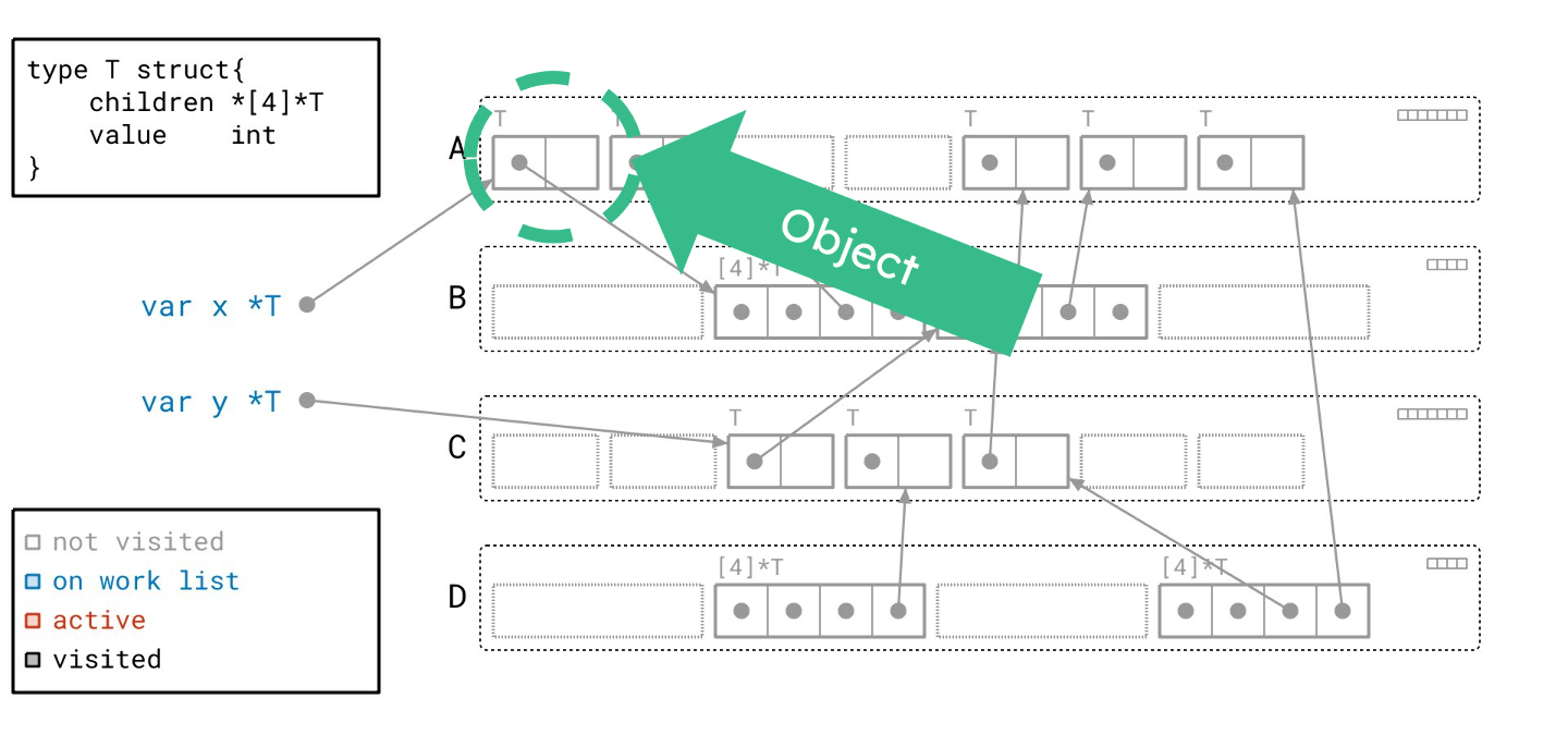
To this end, the Go garbage collector concerns itself with objects and pointers.

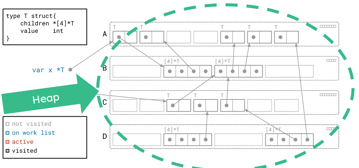
In the context of the Go runtime, objects are Go values whose underlying memory is allocated from the heap. Heap objects are created when the Go compiler can’t figure out how else to allocate memory for a value. For example, the following code snippet allocates a single heap object: the backing store for a slice of pointers.

var x = make([]*int, 10) // global

The Go compiler can’t allocate the slice backing store anywhere except the heap, since it’s very hard, and maybe even impossible, for it to know how long x will refer to the object for.

Pointers are just numbers that indicate the location of a Go value in memory, and they’re how a Go program references objects. For example, to get the pointer to the beginning of the object allocated in the last code snippet, we can write:

&x[0] // 0xc000104000

The mark-sweep algorithm

Go’s garbage collector follows a strategy broadly referred to as tracing garbage collection, which just means that the garbage collector follows, or traces, the pointers in the program to identify which objects the program is still using.

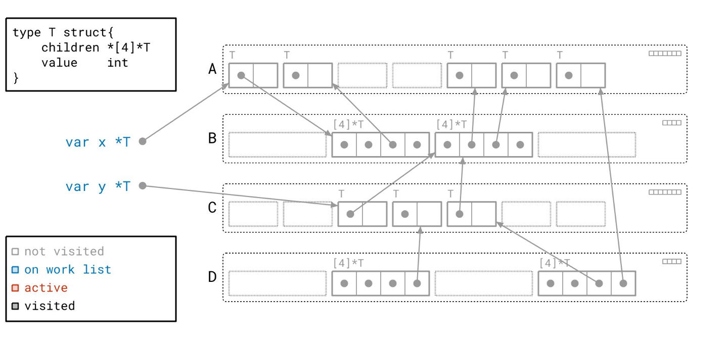
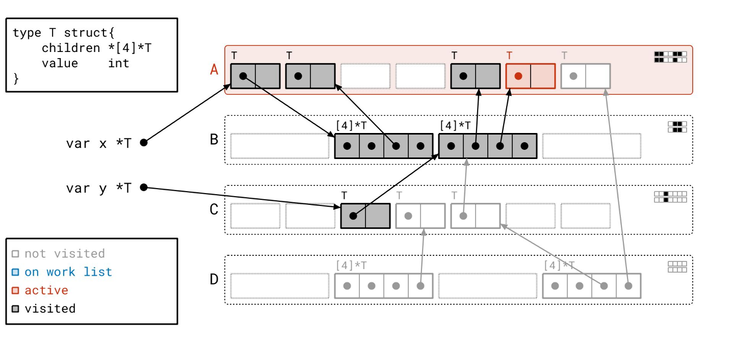
More specifically, the Go garbage collector implements the mark-sweep algorithm. This is much simpler than it sounds. Imagine objects and pointers as a sort of graph, in the computer science sense. Objects are nodes, pointers are edges.

The mark-sweep algorithm operates on this graph, and as the name might suggest, proceeds in two phases.

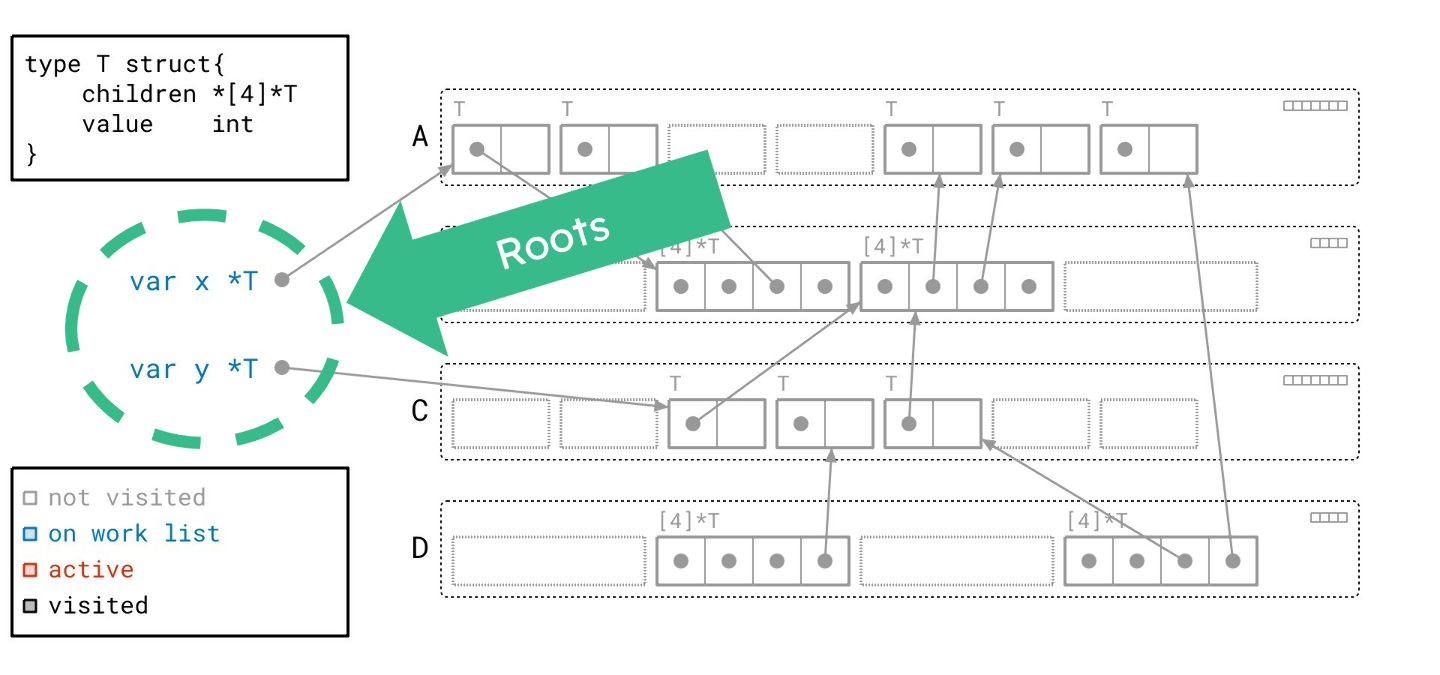
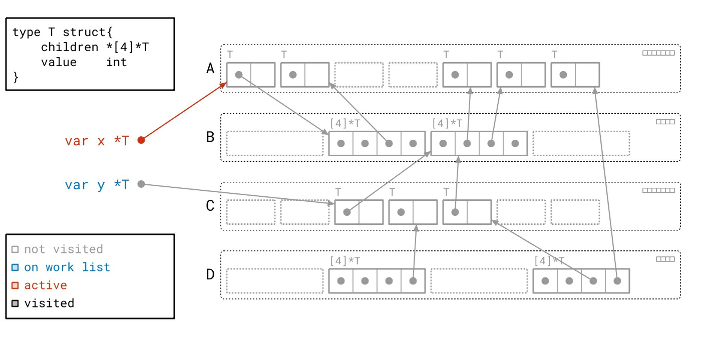
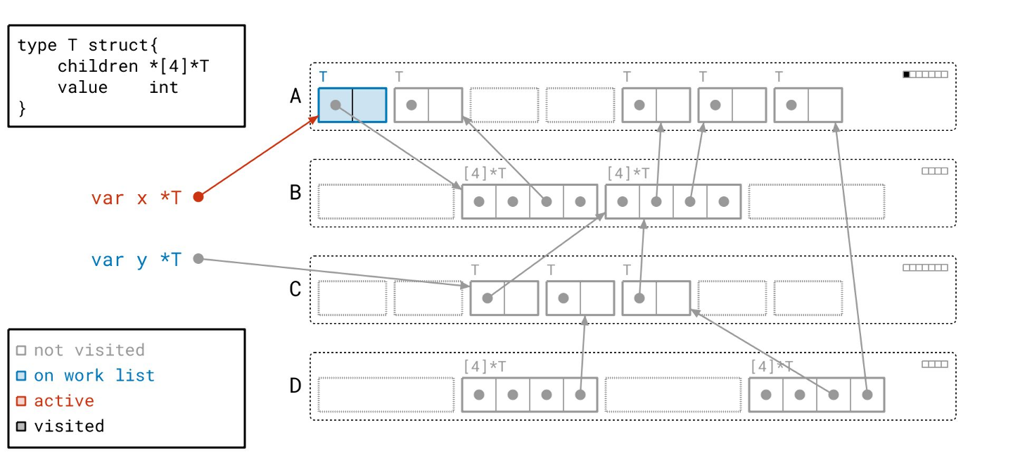
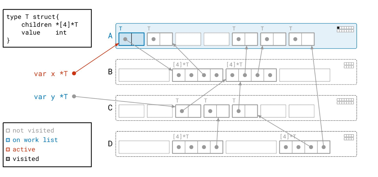
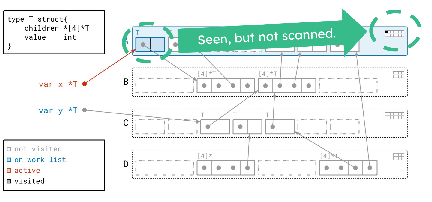
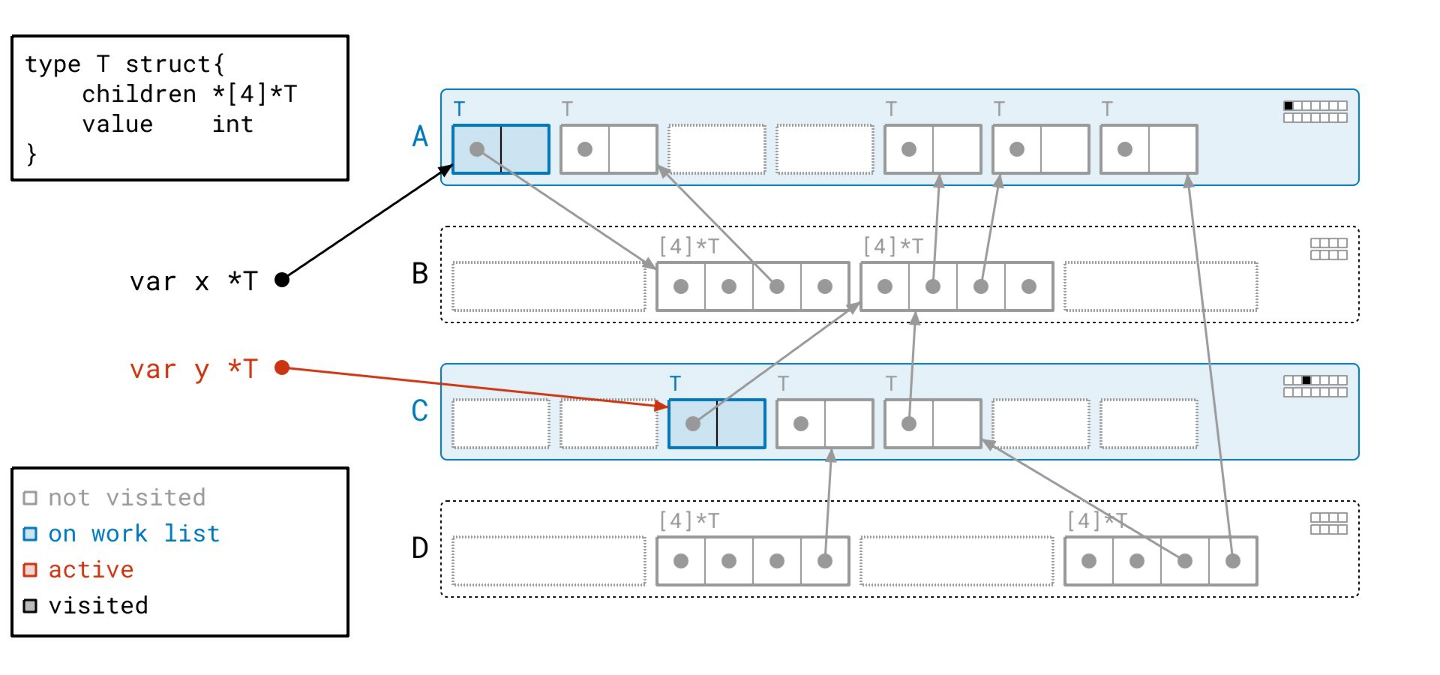
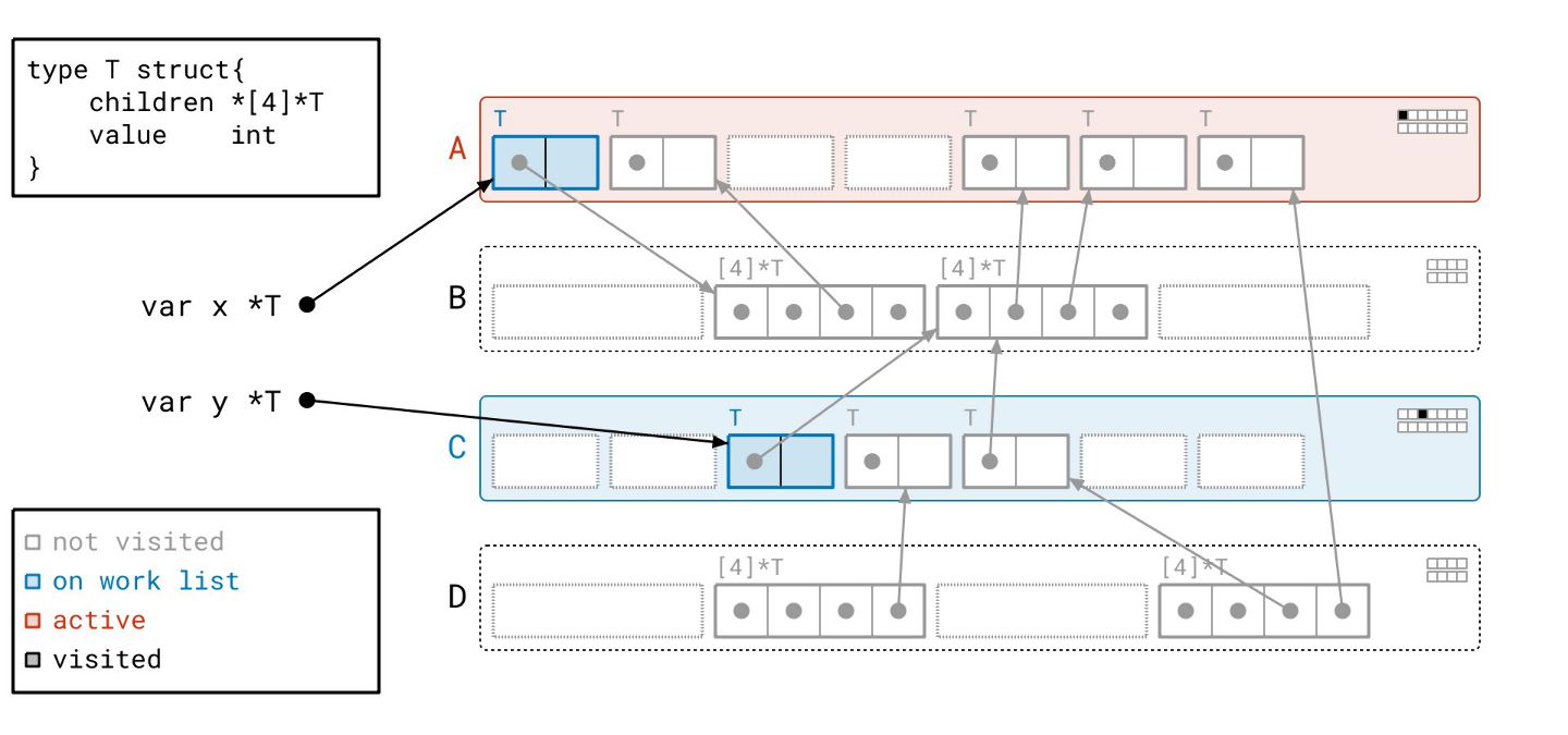
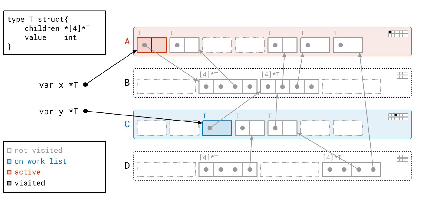
In the first phase, the mark phase, it walks the object graph from well-defined source edges called roots. Think global and local variables. Then, it marks everything it finds along the way as visited, to avoid going in circles. This is analogous to your typical graph flood algorithm, like a depth-first or breadth-first search.

Next is the sweep phase. Whatever objects were not visited in our graph walk are unused, or unreachable, by the program. We call this state unreachable because it is impossible with normal safe Go code to access that memory anymore, simply through the semantics of the language. To complete the sweep phase, the algorithm simply iterates through all the unvisited nodes and marks their memory as free, so the memory allocator can reuse it.

That’s it?

You may think I’m oversimplifying a bit here. Garbage collectors are frequently referred to as magic, and black boxes. And you’d be partially right, there are more complexities.

For example, this algorithm is, in practice, executed concurrently with your regular Go code. Walking a graph that’s mutating underneath you brings challenges. We also parallelize this algorithm, which is a detail that’ll come up again later.

But trust me when I tell you that these details are mostly separate from the core algorithm. It really is just a simple graph flood at the center.

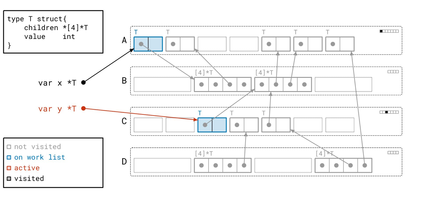
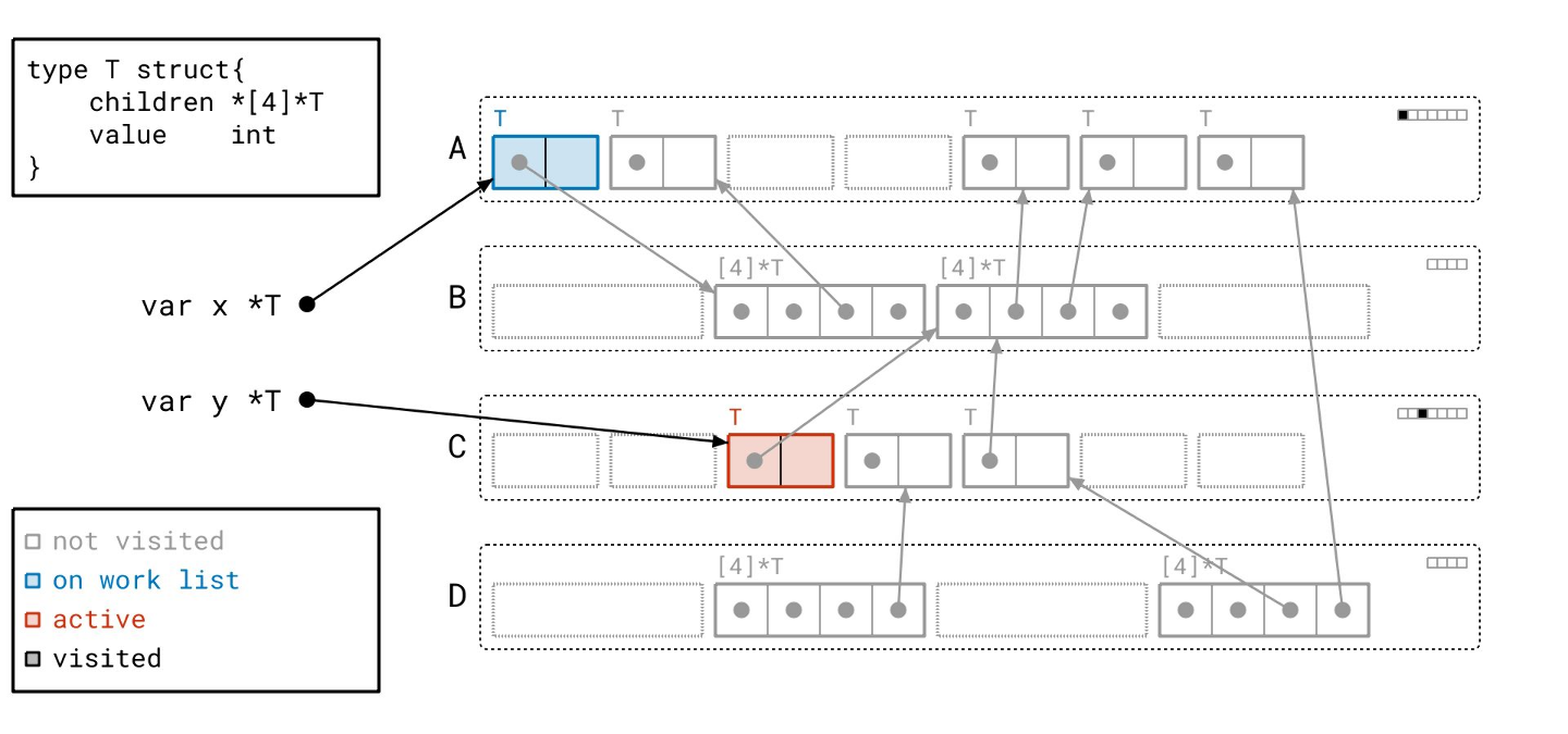
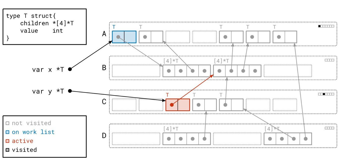
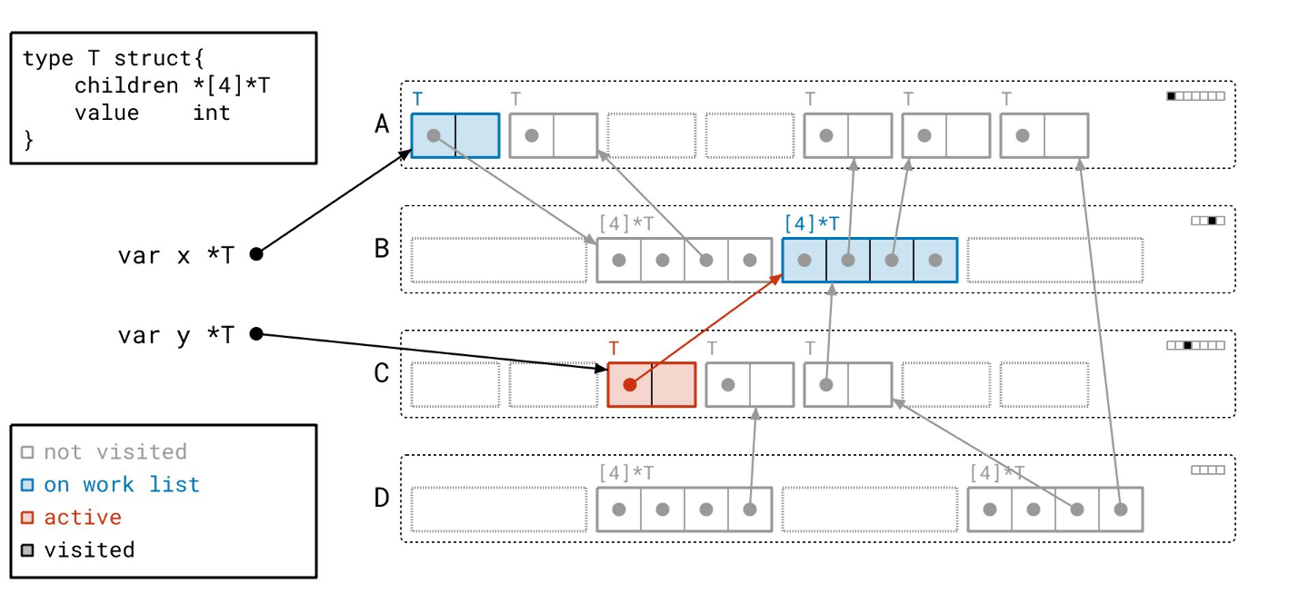
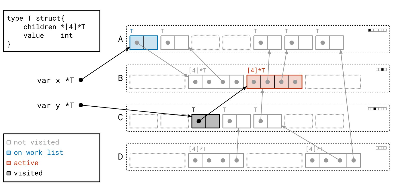
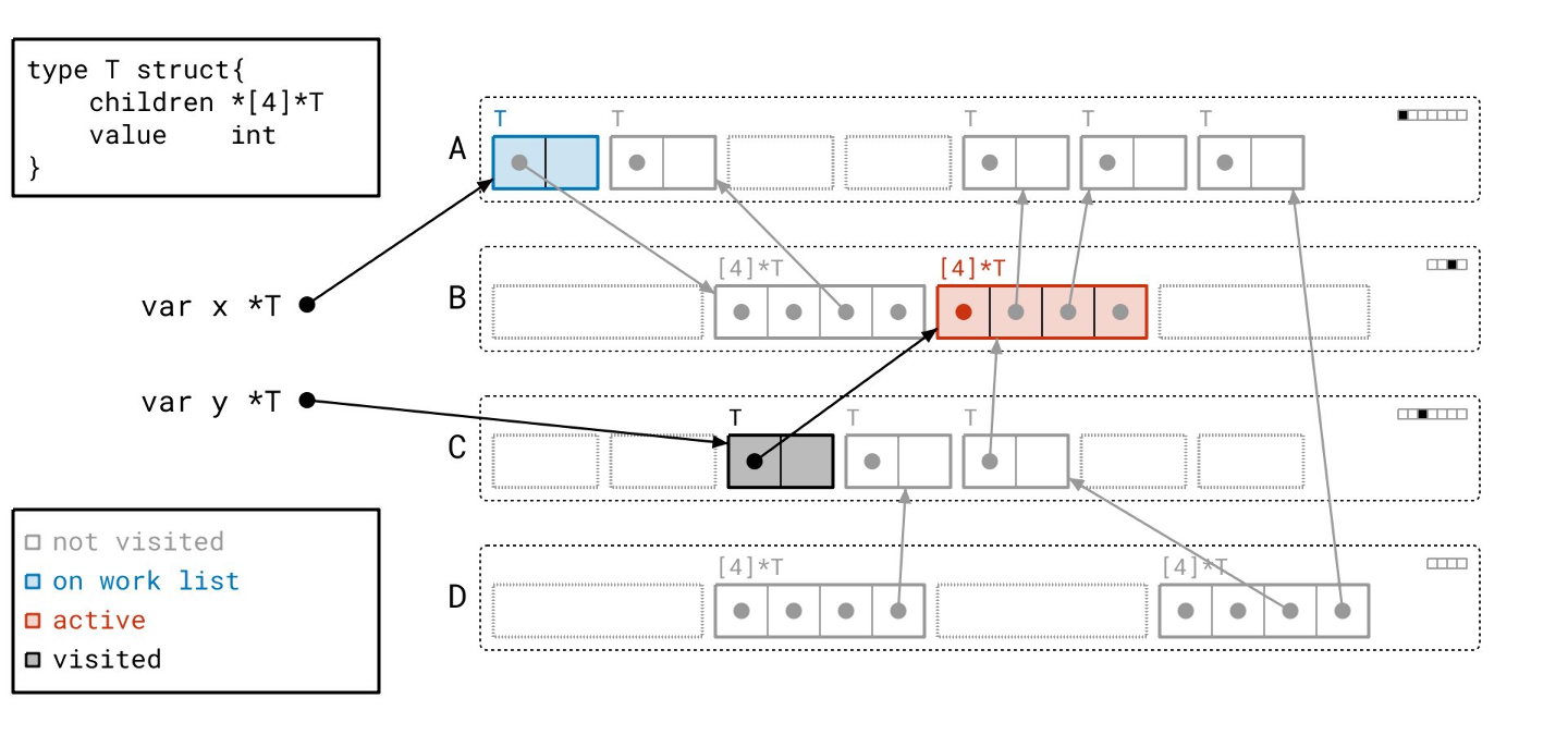
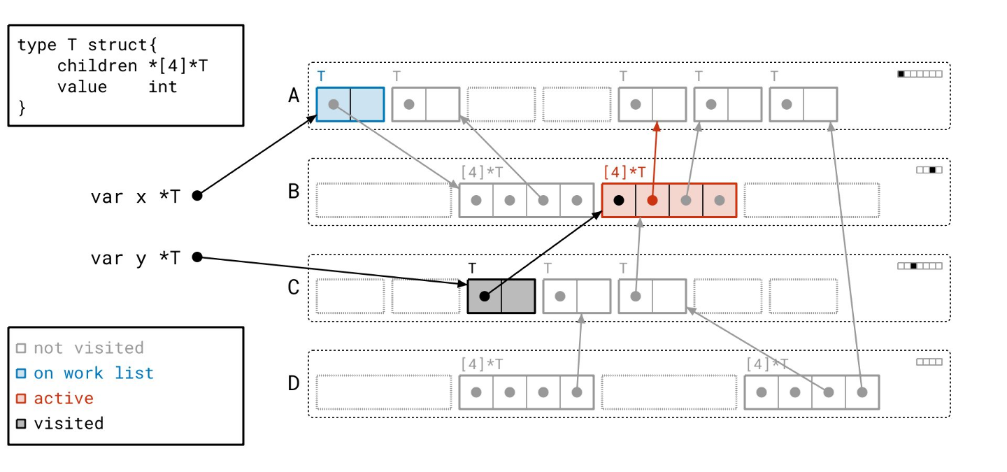
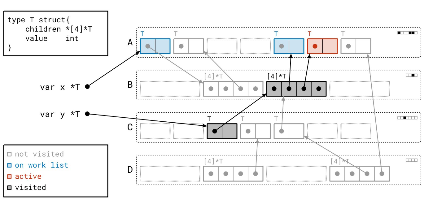
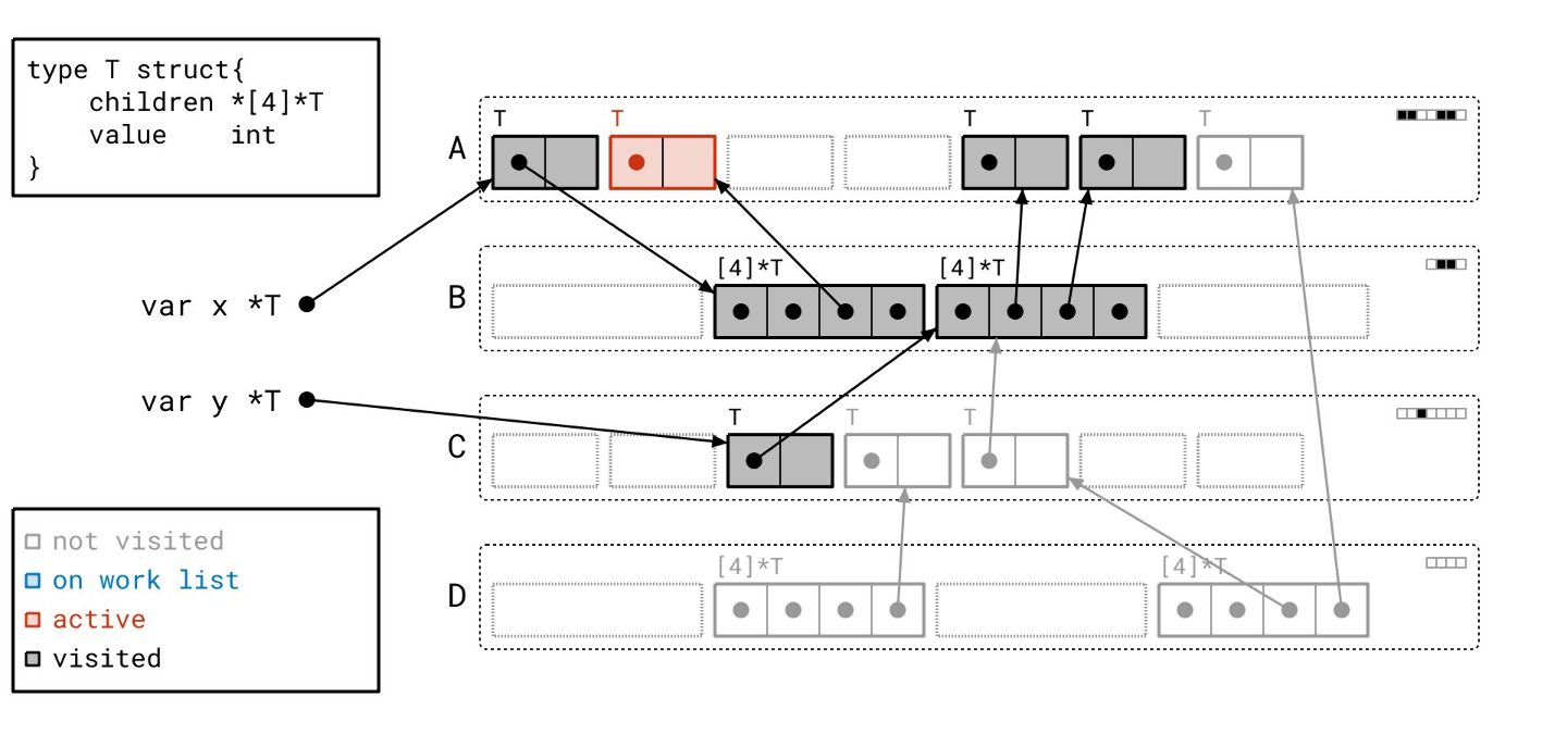
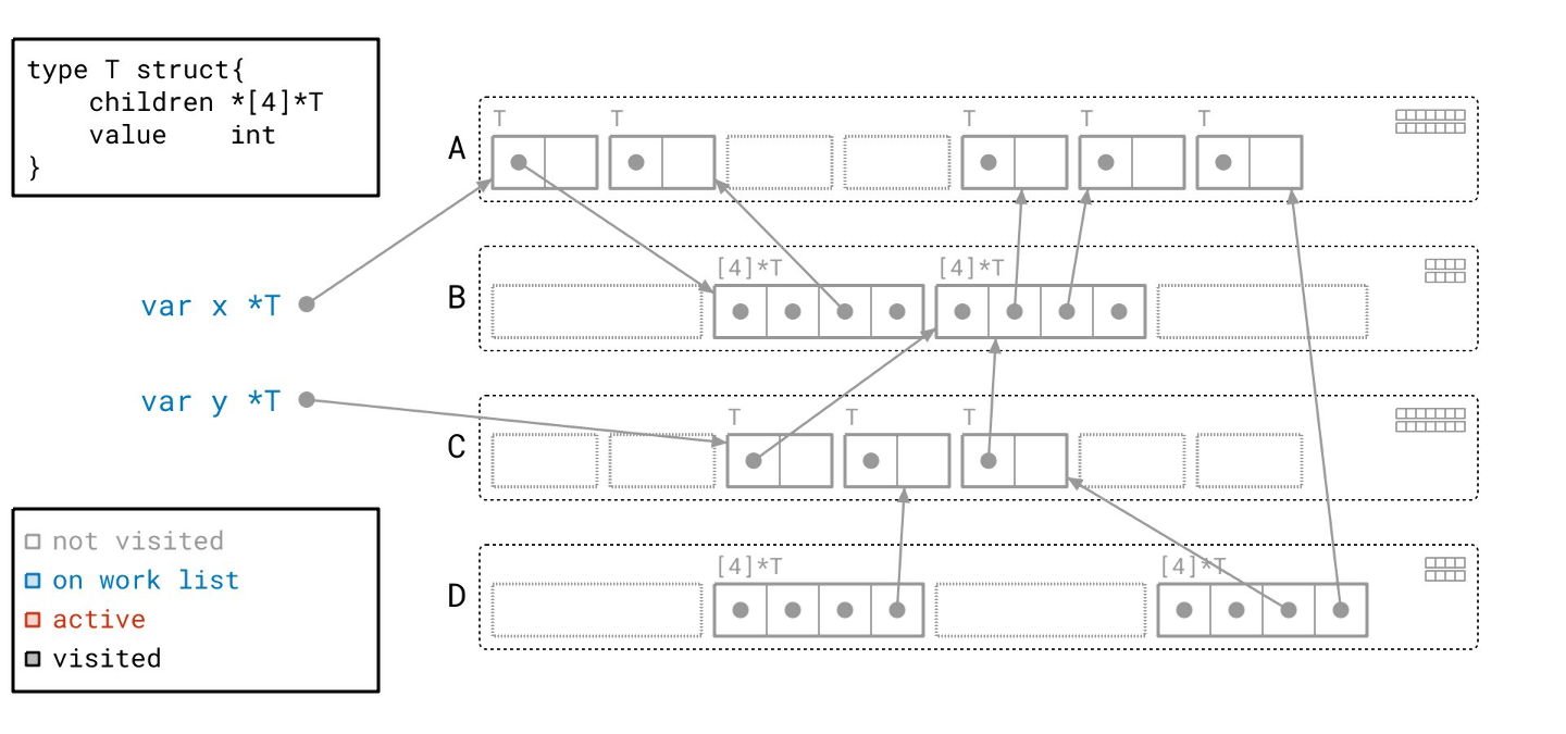
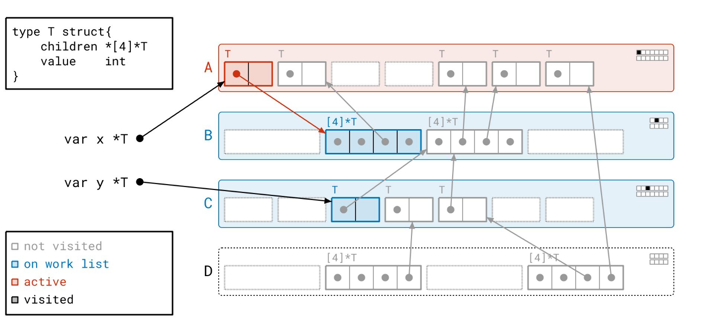
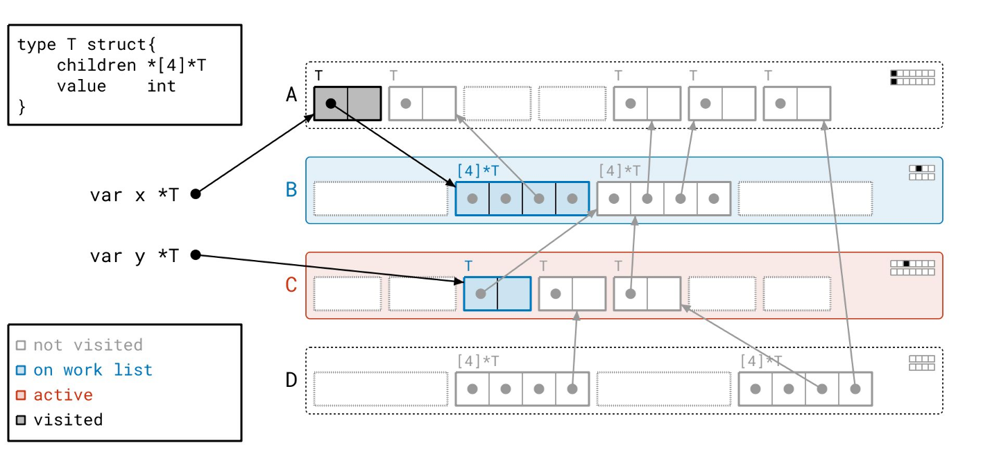
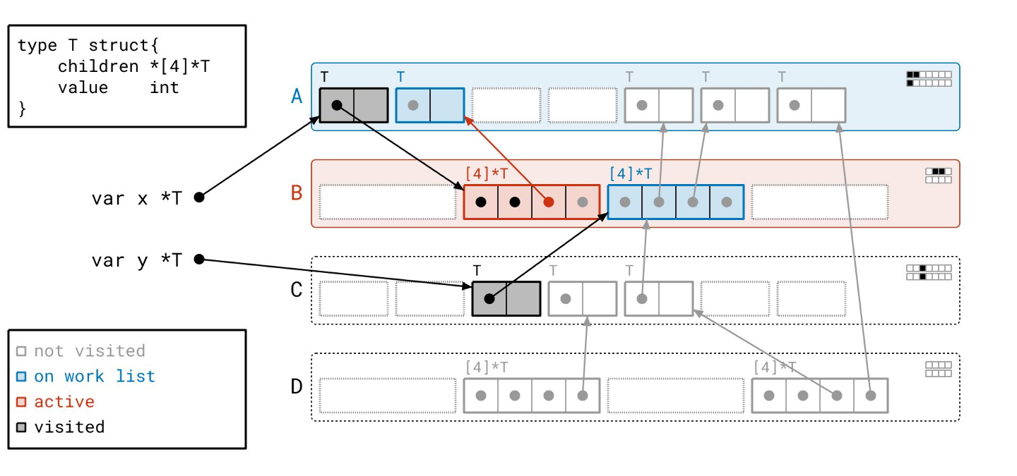
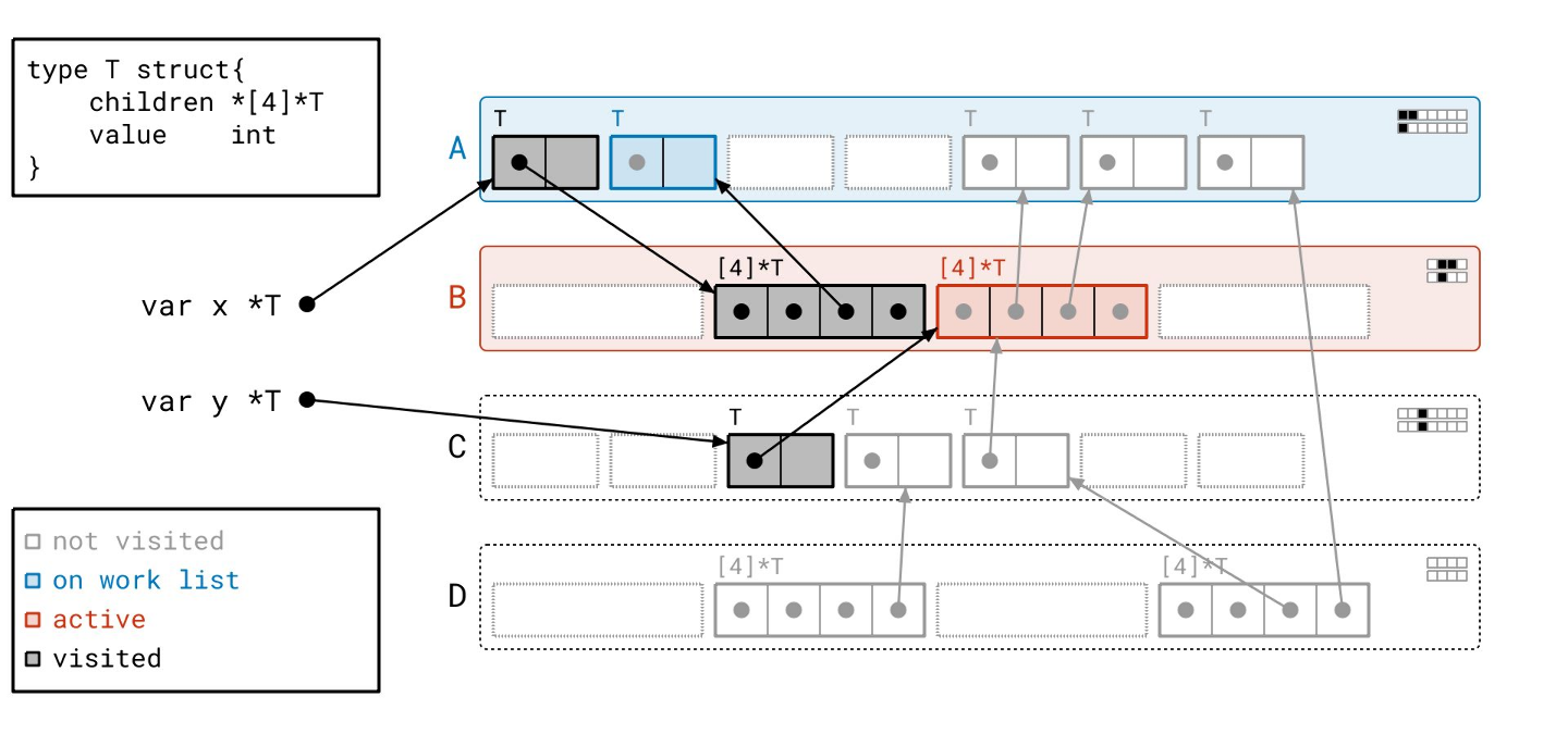
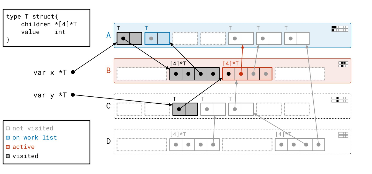
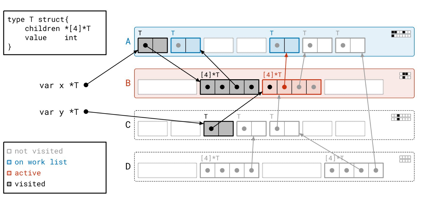
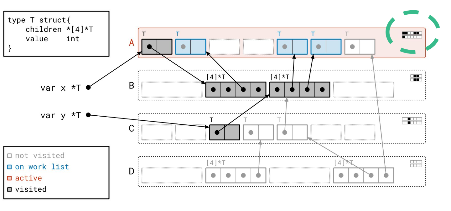
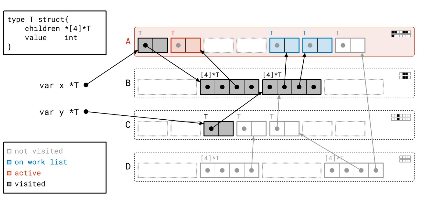
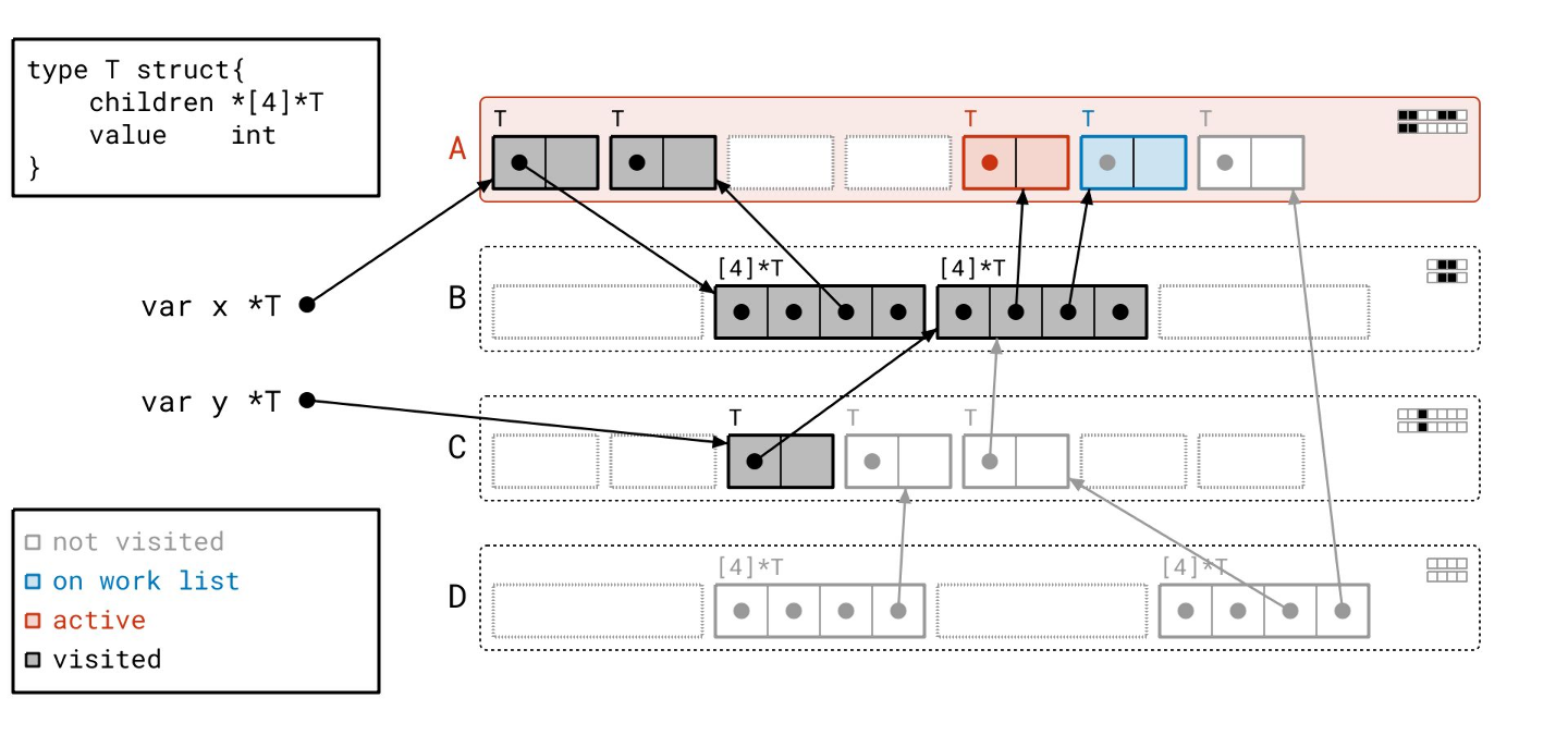
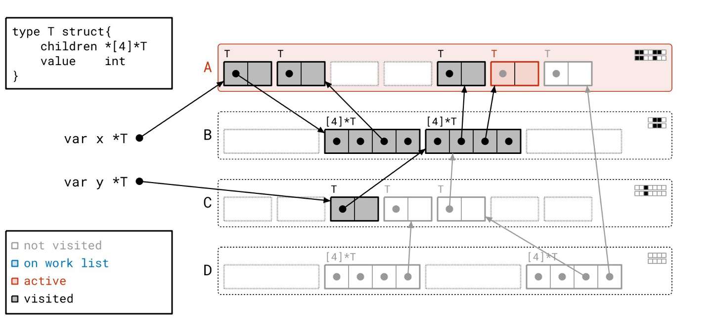
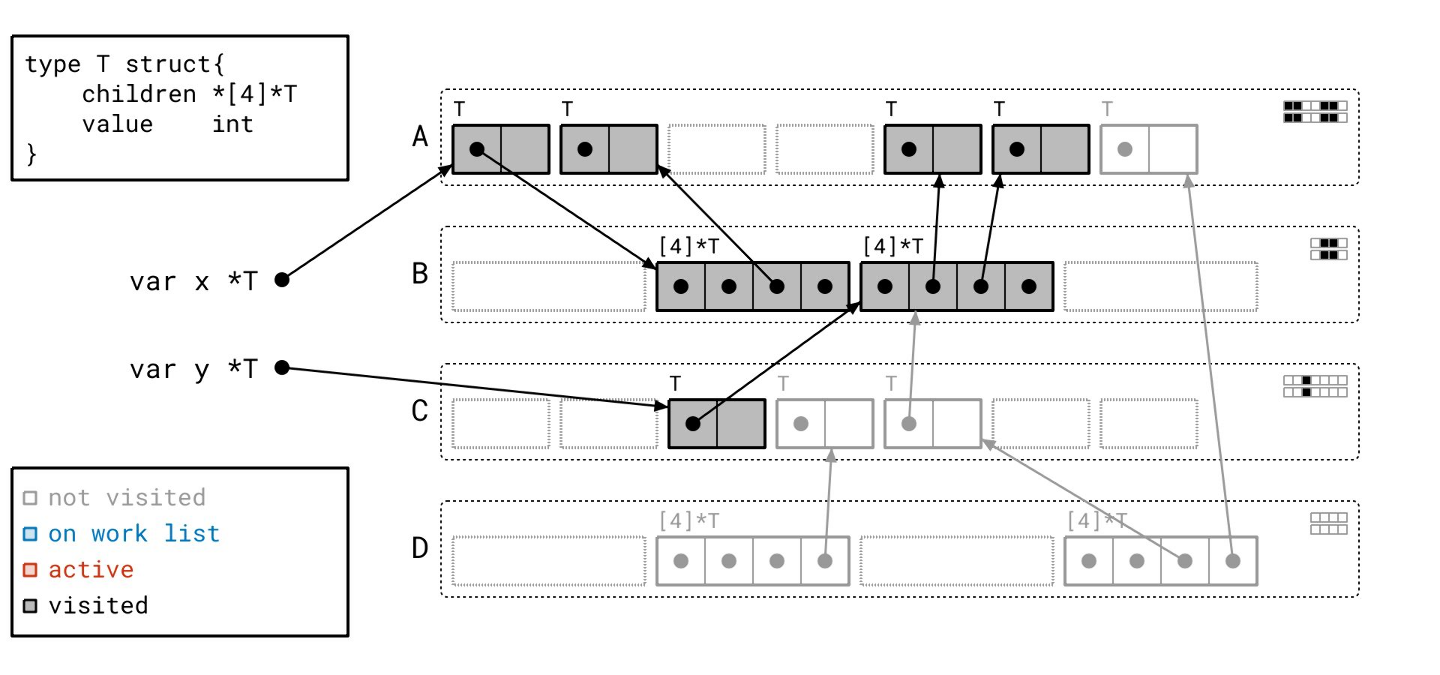
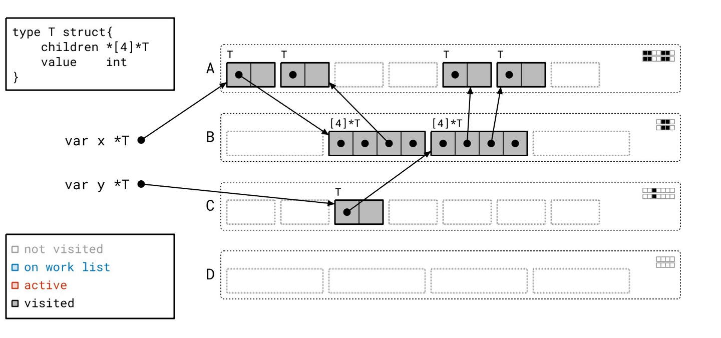
Graph flood example

Let’s walk through an example. Navigate through the slideshow below to follow along.

Scroll horizontally through the slideshow!

Here we have a diagram of some global variables and Go heap. Let's break it down, piece by piece.

On the left here we have our roots. These are global variables x and y. They will be the starting point of our graph walk. Since they're marked blue, according to our handy legend in the bottom left, they're currently on our work list.

On the right side, we have our heap. Currently, everything in our heap is grayed out because we haven't visited any of it yet.

Each one of these rectangles represents an object. Each object is labeled with its type. This object in particular is an object of type T, whose type definition is on the top left. It's got a pointer to an array of children, and some value. We can surmise that this is some kind of recursive tree data structure.

In addition to the objects of type T, you'll also notice that we have array objects containing *Ts. These are pointed to by the "children" field of objects of type T.

Each square inside of the rectangle represents 8 bytes of memory. A square with a dot is a pointer. If it has an arrow, it is a non-nil pointer pointing to some other object.

And if it doesn't have a corresponding arrow, then it's a nil pointer.

Next, these dotted rectangles represents free space, what I'll call a free "slot." We could put an object there, but there currently isn't one.

You'll also notice that objects are grouped together by these labeled, dotted rounded rectangles. Each of these represents a page: a contiguous block of memory. These pages are labeled A, B, C, and D, and I'll refer to them that way.

In this diagram, each object is allocated as part of some page. Like in the real implementation, each page here only contains objects of a certain size. This is just how the Go heap is organized.

Pages are also how we organize per-object metadata. Here you can see seven boxes, each corresponding to one of the seven object slots in page A.

Each box represents one bit of information: whether or not we have seen the object before. This is actually how the real runtime manages whether an object has been visited, and it'll be an important detail later.

That was a lot of detail, so thanks for reading along. This will all come into play later. For now, let's just see how our graph flood applies to this picture.

We start by taking a root off of the work list. We mark it red to indicate that it's now active.

Following that root's pointer, we find an object of type T, which we add to our work list. Following our legend, we draw the object in blue to indicate that it's on our work list. Note also that we set the seen bit corresponding to this object in our metadata.

Now that we've taken care of all the roots, we're left with two objects on our work list. Let's take an object off the work list.

What we're going to do now is walk the pointers of the objects, to find more objects. By the way, we call walking the pointers of an object "scanning" the object.

Then we walk the objects that the array object referred to!

And note that we still have to walk over all pointers, even if they're nil. We don't know ahead of time if they will be.

And now we've reached the other branch, starting from that object in page A we found much earlier from one of the roots.

You may be noticing a last-in-first-out discipline for our work list here, indicating that our work list is a stack, and hence our graph flood is approximately depth-first. This is intentional, and reflects the actual graph flood algorithm in the Go runtime.

Just one more object left on our work list…

And we're done with the mark phase! There's nothing we're actively working on and there's nothing left on our work list. Every object drawn in black is reachable, and every object drawn in gray is unreachable. Let's sweep the unreachable objects, all in one go.

We've converted those objects into free slots, ready to hold new objects.

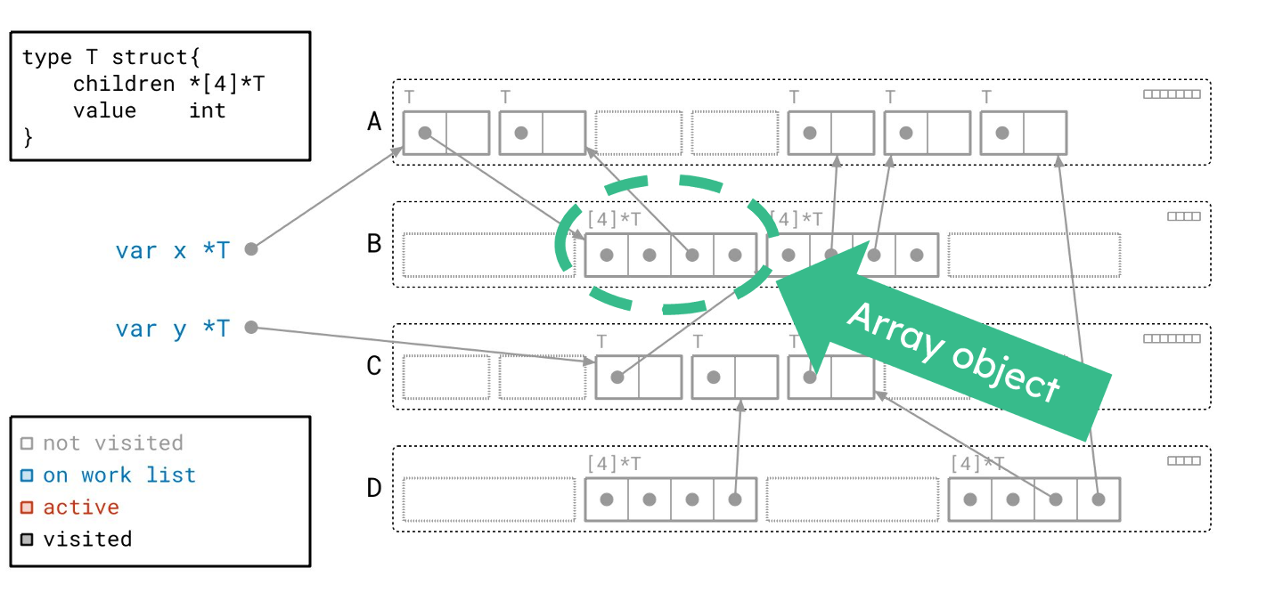
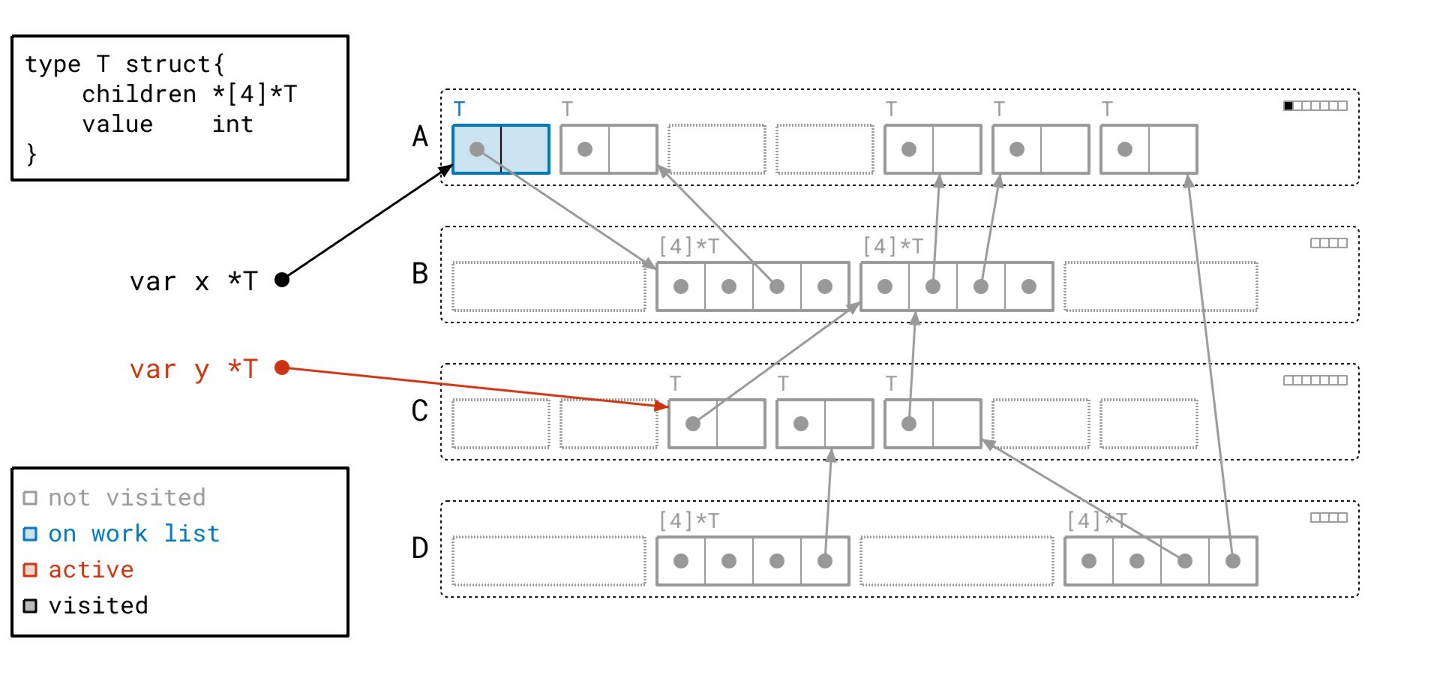
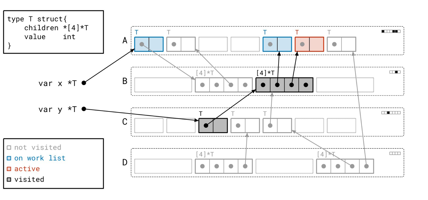
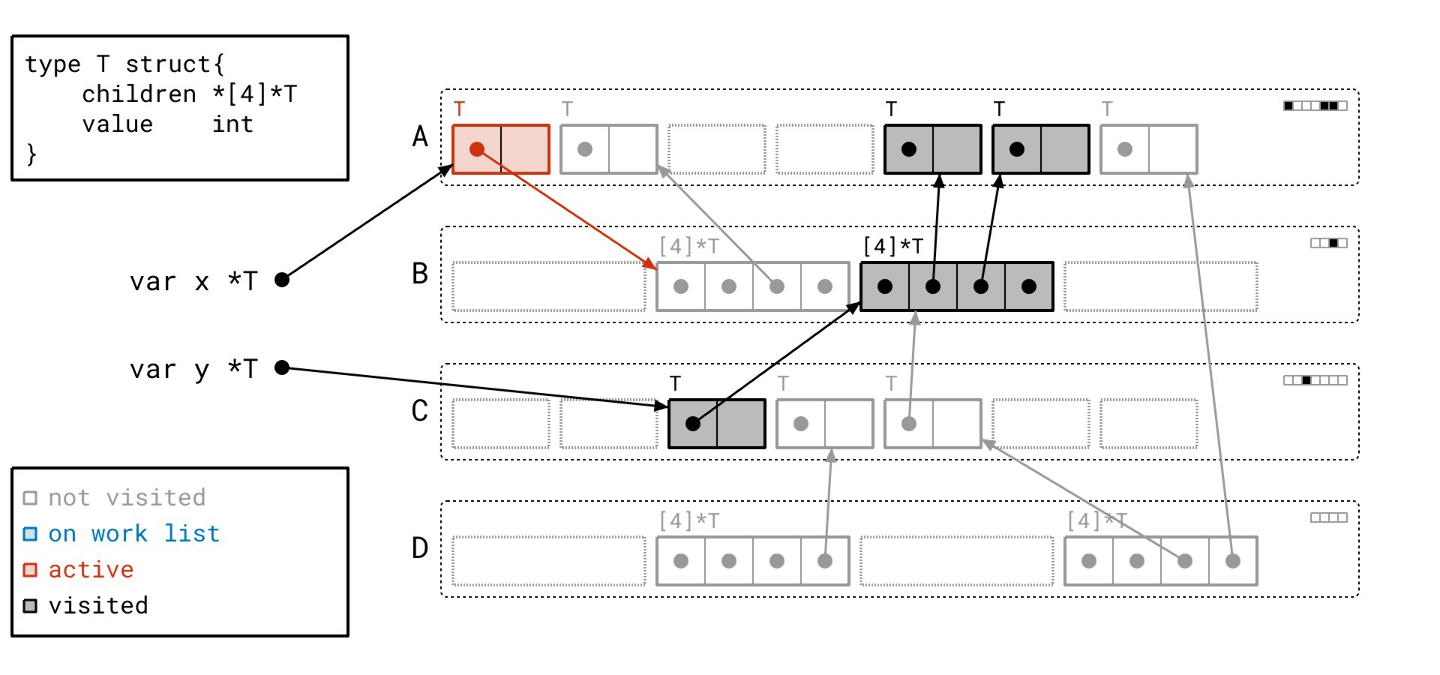
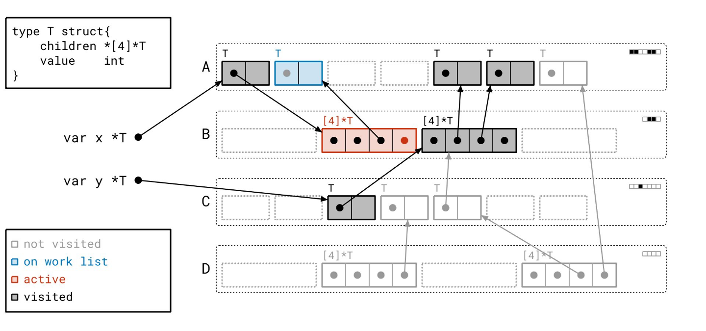
The problem

After all that, I think we have a handle on what the Go garbage collector is actually doing. This process seems to work well enough today, so what’s the problem?

Well, it turns out we can spend a lot of time executing this particular algorithm in some programs, and it adds substantial overhead to nearly every Go program. It’s not that uncommon to see Go programs spending 20% or more of their CPU time in the garbage collector.

Let’s break down where that time is being spent.

Garbage collection costs

At a high level, there are two parts to the cost of the garbage collector. The first is how often it runs, and the second is how much work it does each time it runs. Multiply those two together, and you get the total cost of the garbage collector.

Total GC cost = Number of GC cycles × Average cost per GC cycle

Over the years we’ve tackled both terms in this equation, and for more on how often the garbage collector runs, see Michael’s GopherCon EU talk from 2022 about memory limits. The guide to the Go garbage collector also has a lot to say about this topic, and is worth a look if you want to dive deeper.

But for now let’s focus only on the second part, the cost per cycle.

From years of poring over CPU profiles to try to improve performance, we know two big things about Go’s garbage collector.

The first is that about 90% of the cost of the garbage collector is spent marking, and only about 10% is sweeping. Sweeping turns out to be much easier to optimize than marking, and Go has had a very efficient sweeper for many years.

The second is that, of that time spent marking, a substantial portion, usually at least 35%, is simply spent stalled on accessing heap memory. This is bad enough on its own, but it completely gums up the works on what makes modern CPUs actually fast.

“A microarchitectural disaster”

What does “gum up the works” mean in this context? The specifics of modern CPUs can get pretty complicated, so let’s use an analogy.

Imagine the CPU driving down a road, where that road is your program. The CPU wants to ramp up to a high speed, and to do that it needs to be able to see far ahead of it, and the way needs to be clear. But the graph flood algorithm is like driving through city streets for the CPU. The CPU can’t see around corners and it can’t predict what’s going to happen next. To make progress, it constantly has to slow down to make turns, stop at traffic lights, and avoid pedestrians. It hardly matters how fast your engine is because you never get a chance to get going.

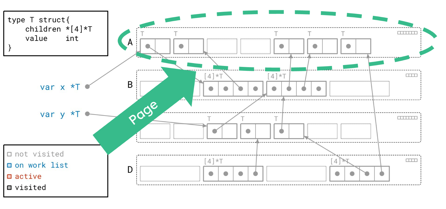
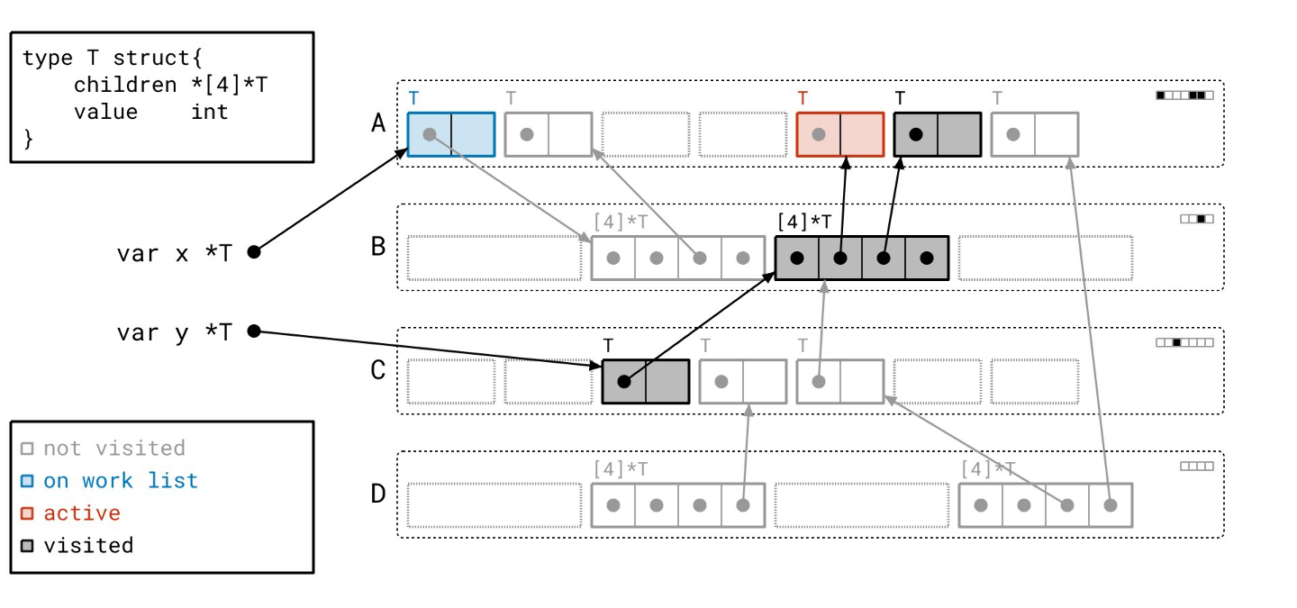
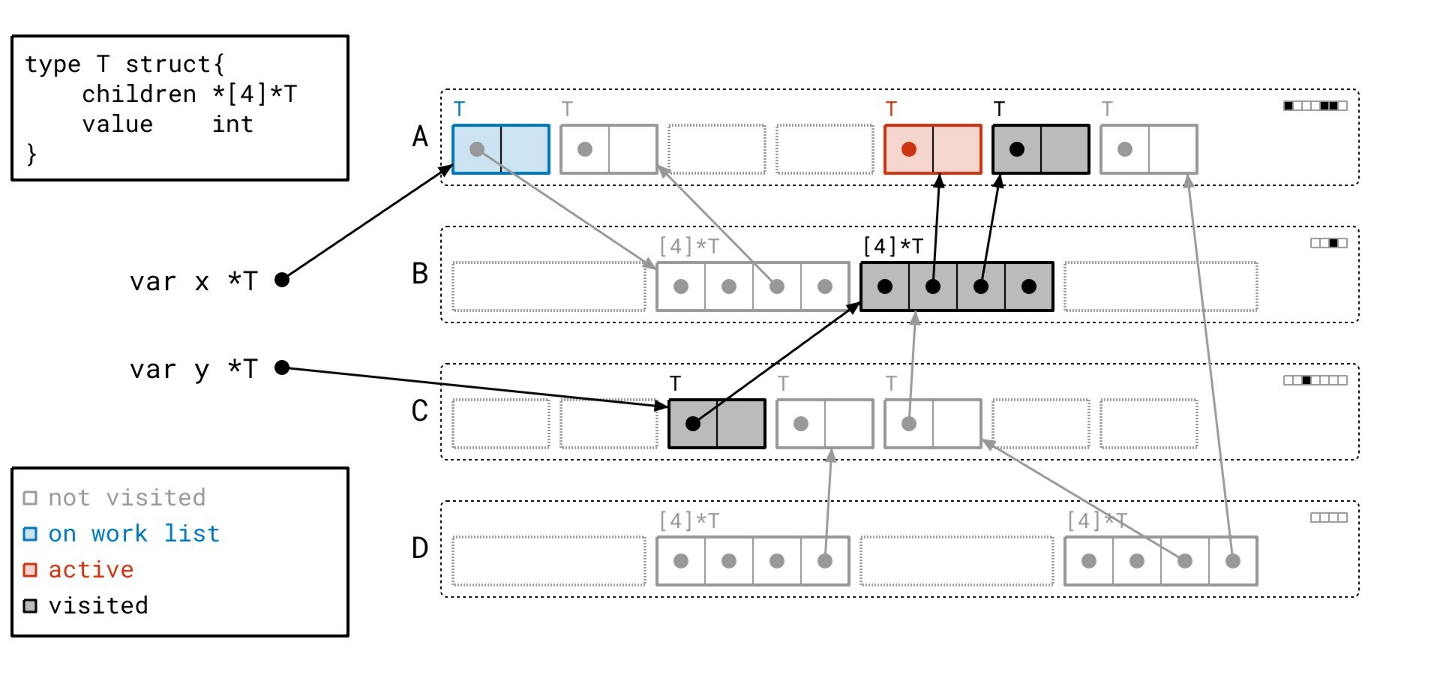
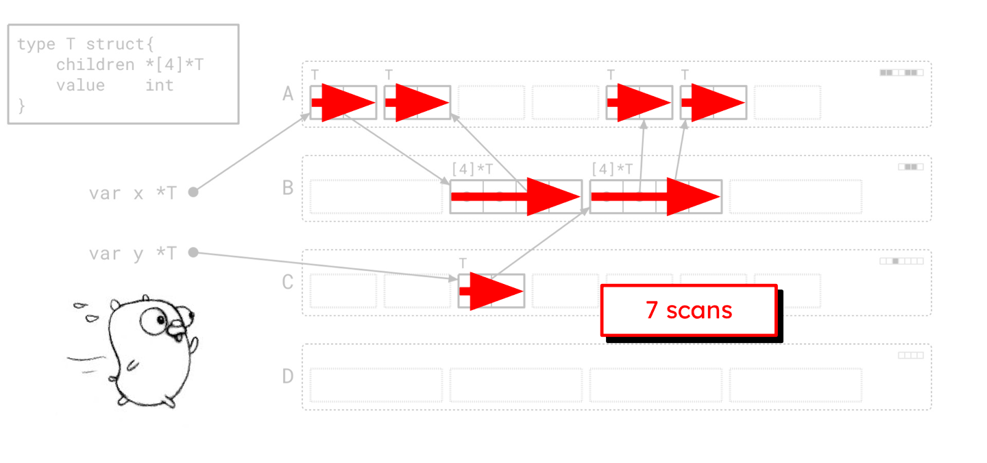
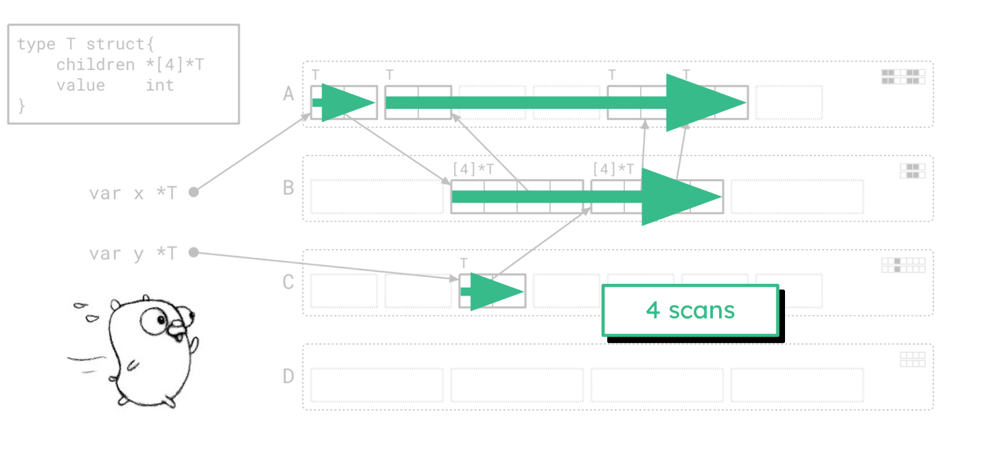
Let’s make that more concrete by looking at our example again. I’ve overlaid the heap here with the path that we took. Each left-to-right arrow represents a piece of scanning work that we did and the dashed arrows show how we jumped around between bits of scanning work.

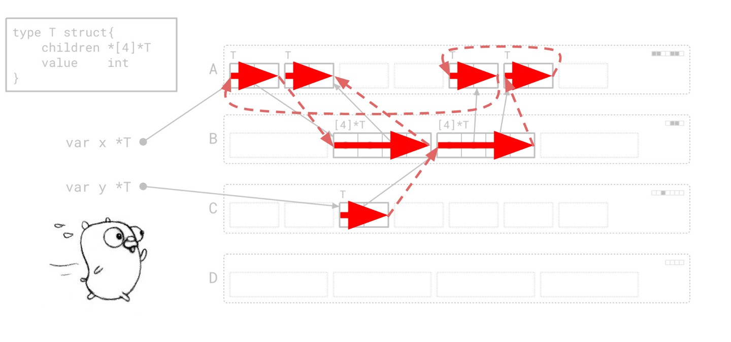
The path through the heap the garbage collector took in our graph flood example.

Notice that we were jumping all over memory doing tiny bits of work in each place. In particular, we’re frequently jumping between pages, and between different parts of pages.

Modern CPUs do a lot of caching. Going to main memory can be up to 100x slower than accessing memory that’s in our cache. CPU caches are populated with memory that’s been recently accessed, and memory that’s nearby to recently accessed memory. But there’s no guarantee that any two objects that point to each other will also be close to each other in memory. The graph flood doesn’t take this into account.

Quick side note: if we were just stalling fetches to main memory, it might not be so bad. CPUs issue memory requests asynchronously, so even slow ones could overlap if the CPU could see far enough ahead. But in the graph flood, every bit of work is small, unpredictable, and highly dependent on the last, so the CPU is forced to wait on nearly every individual memory fetch.

And unfortunately for us, this problem is only getting worse. There’s an adage in the industry of “wait two years and your code will get faster.”

But Go, as a garbage collected language that relies on the mark-sweep algorithm, risks the opposite. “Wait two years and your code will get slower.” The trends in modern CPU hardware are creating new challenges for garbage collector performance:

Non-uniform memory access. For one, memory now tends to be associated with subsets of CPU cores. Accesses by other CPU cores to that memory are slower than before. In other words, the cost of a main memory access depends on which CPU core is accessing it. It’s non-uniform, so we call this non-uniform memory access, or NUMA for short.

Reduced memory bandwidth. Available memory bandwidth per CPU is trending downward over time. This just means that while we have more CPU cores, each core can submit relatively fewer requests to main memory, forcing non-cached requests to wait longer than before.

Ever more CPU cores. Above, we looked at a sequential marking algorithm, but the real garbage collector performs this algorithm in parallel. This scales well to a limited number of CPU cores, but the shared queue of objects to scan becomes a bottleneck, even with careful design.

Modern hardware features. New hardware has fancy features like vector instructions, which let us operate on a lot of data at once. While this has the potential for big speedups, it’s not immediately clear how to make that work for marking because marking does so much irregular and often small pieces of work.

Green Tea

Finally, this brings us to Green Tea, our new approach to the mark-sweep algorithm. The key idea behind Green Tea is astonishingly simple:

Work with pages, not objects.

Sounds trivial, right? And yet, it took a lot of work to figure out how to order the object graph walk and what we needed to track to make this work well in practice.

More concretely, this means:

Instead of scanning objects we scan whole pages.
Instead of tracking objects on our work list, we track whole pages.
We still need to mark objects at the end of the day, but we’ll track marked objects locally to each page, rather than across the whole heap.

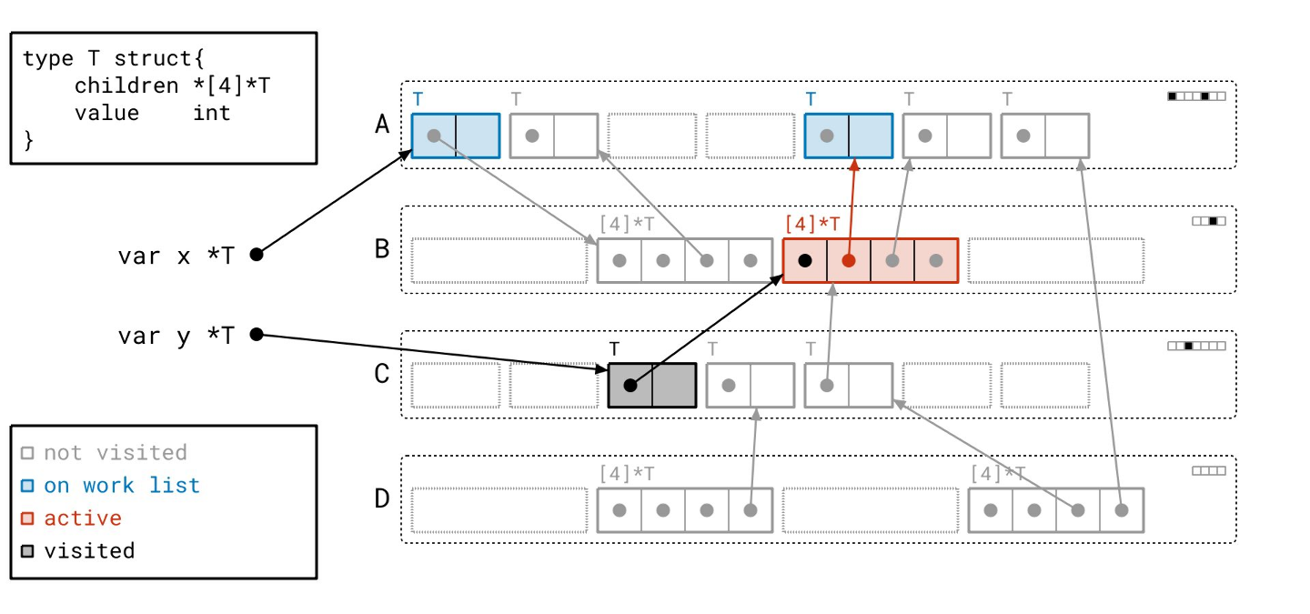
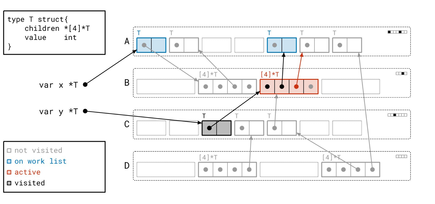
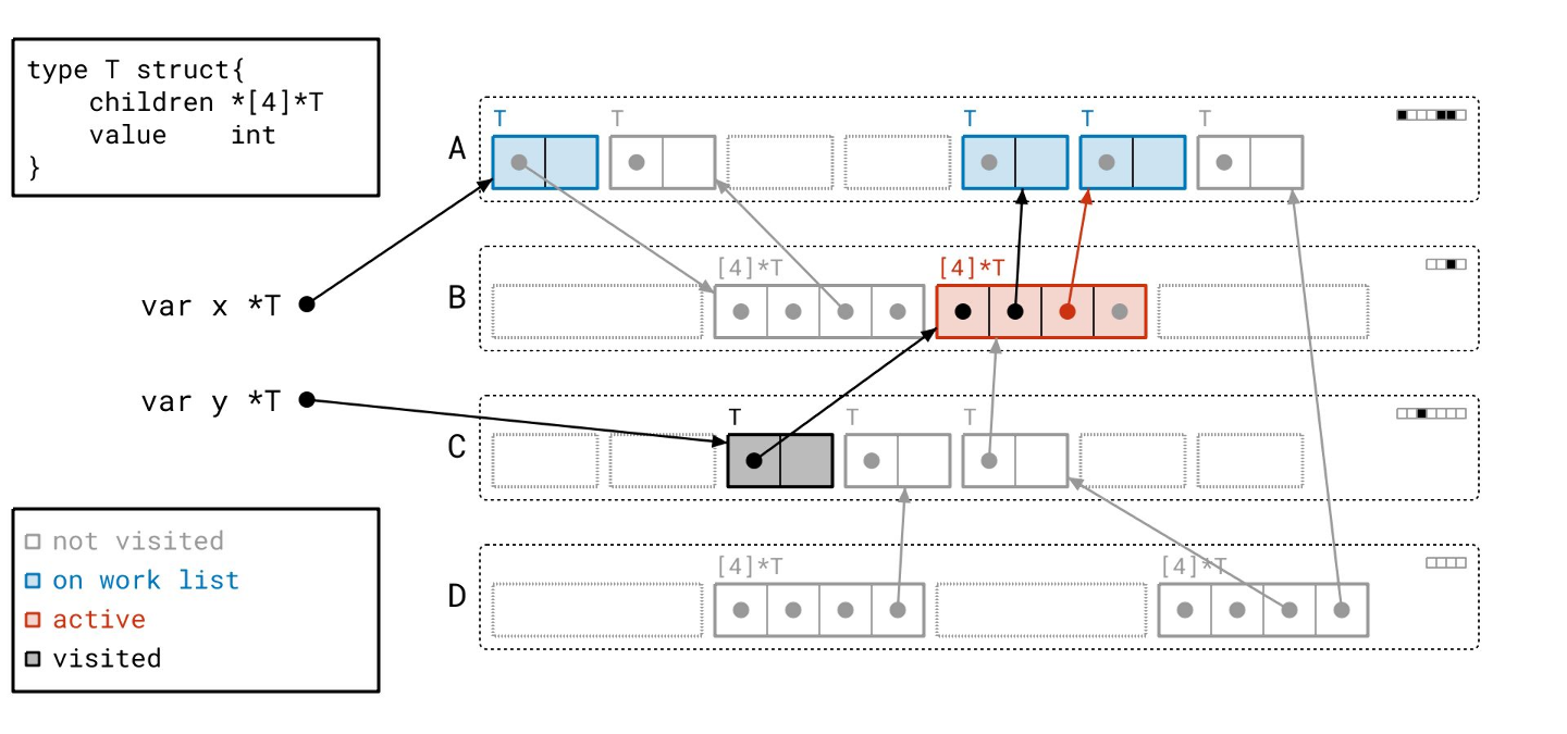
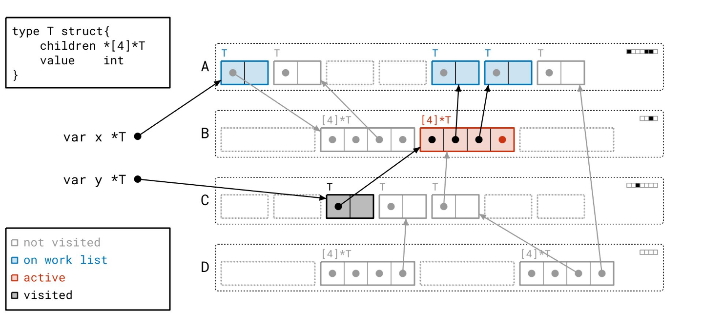
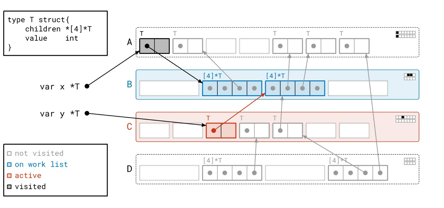
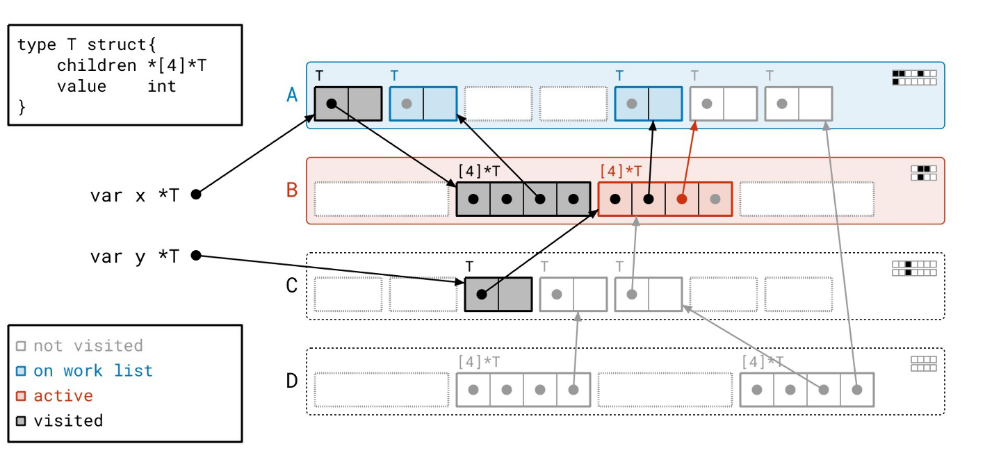
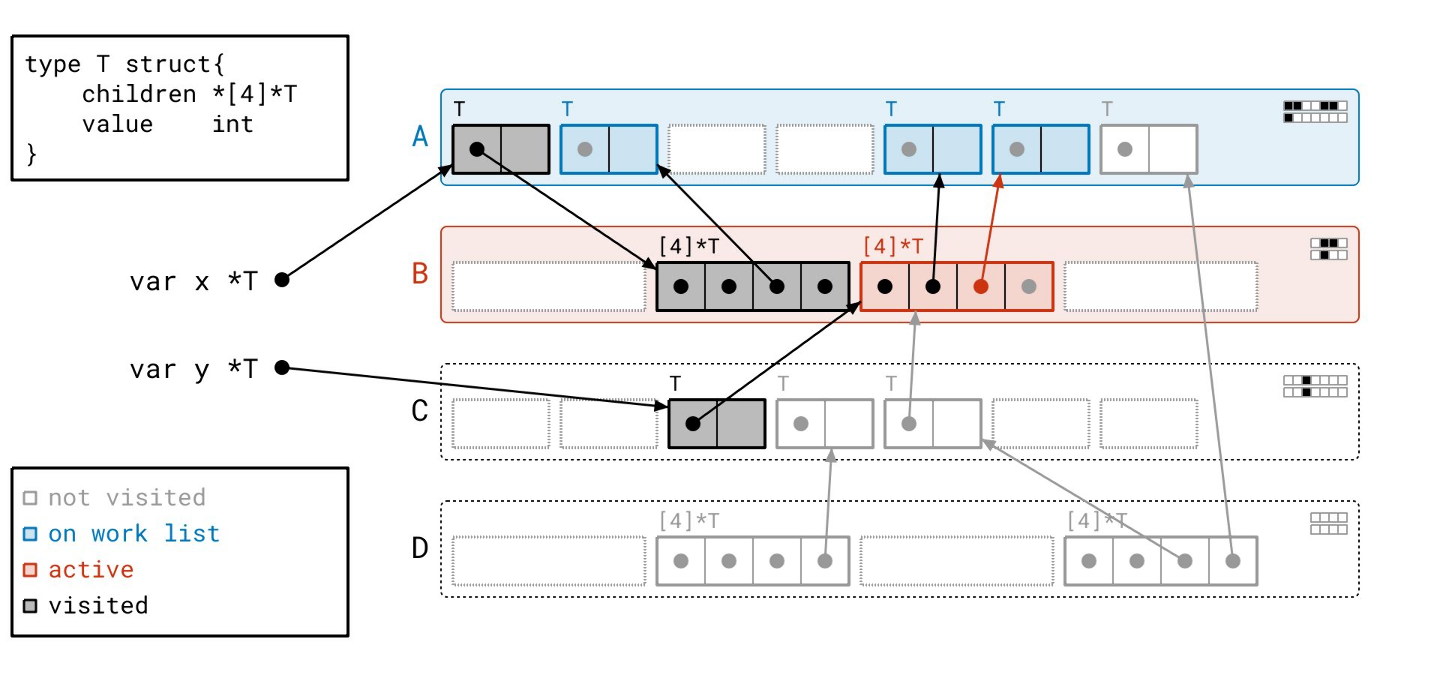
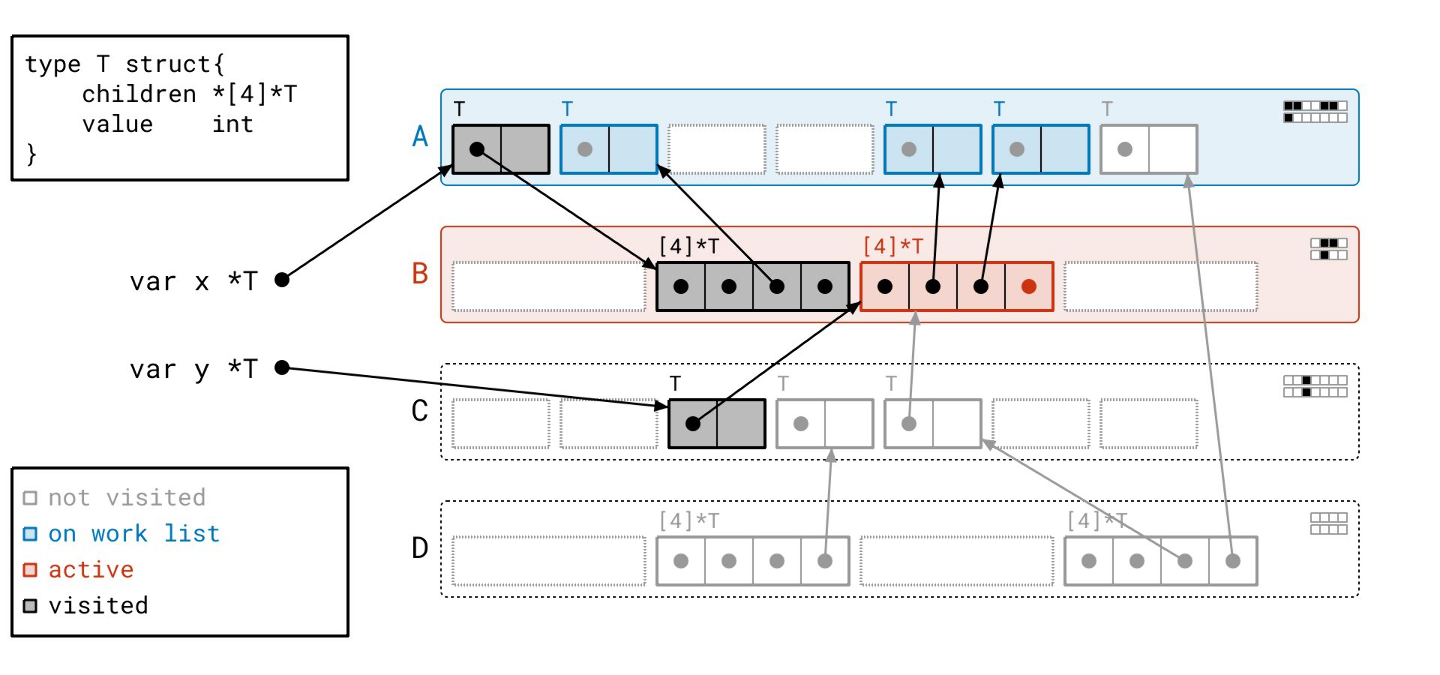
Green Tea example

Let’s see what this means in practice by looking at our example heap again, but this time running Green Tea instead of the straightforward graph flood.

As above, navigate through the annotated slideshow to follow along.

Scroll horizontally through the slideshow!

This is the same heap as before, but now with two bits of metadata per object rather than one. Again, each bit, or box, corresponds to one of the object slots in the page. In total, we now have fourteen bits that correspond to the seven slots in page A.

The top bits represent the same thing as before: whether or not we've seen a pointer to the object. I'll call these the "seen" bits. The bottom set of bits are new. These "scanned" bits track whether or not we've *scanned* the object.

This new piece of metadata is necessary because, in Green tea, **the work list tracks pages, not objects**. We still need to track objects at some level, and that's the purpose of these bits.

We start off the same as before, walking objects from the roots.

But this time, instead of putting an object on the work list, we put a whole page–in this case page A–on the work list, indicated by shading the whole page blue.

The object we found is also blue to indicate that when we do take this page off of the work list, we will need to look at that object. Note that the object's blue hue directly reflects the metadata in page A. Its corresponding seen bit is set, but its scanned bit is not.

We follow the next root, find another object, and again put the whole page–page C–on the work list and set the object's seen bit.

We're done following roots, so we turn to the work list and take page A off the work list.

Using the seen and scanned bits, we can tell there's one object to scan on page A.

We scan that object, following its pointers. And as a result, we add page B to the work list, since the first object in page A points to an object in page B.

We're done with page A. Next we take page C off the work list.

Similar to page A, there's a single object on page C to scan.

We found a pointer to another object in page B. Page B is already on the work list, so we don't need to add anything to the work list. We simply have to set the seen bit for the target object.

Now it's page B's turn. We've accumulated two objects to scan on page B, and we can process both of these objects in a row, in memory order!

We walk the pointers of the first object…

We find a pointer to an object in page A. Page A was previously on the work list, but isn't at this point, so we put it back on the work list. Unlike the original mark-sweep algorithm, where any given object is only added to the work list at most once per whole mark phase, in Green Tea, a given page can reappear on the work list several times during a mark phase.

We scan the second seen object in the page immediately after the first.

We're done scanning page B, so we pull page A off the work list.

This time we only need to scan three objects, not four, since we already scanned the first object. We know which objects to scan by looking at the difference between the "seen" and "scanned" bits.

We're done! There are no more pages on the work list and there's nothing we're actively looking at. Notice that the metadata now all lines up nicely, since all reachable objects were both seen and scanned.

You may have also noticed during our traversal that the work list order is a little different from the graph flood. Where the graph flood had a last-in-first-out, or stack-like, order, here we're using a first-in-first-out, or queue-like, order for the pages on our work list.

This is intentional. We let seen objects accumulate on each page while the page sits on the queue, so we can process as many as we can at once. That's how we were able to hit so many objects on page A at once. Sometimes laziness is a virtue.

And finally we can sweep away the unvisited objects, as before.

Getting on the highway

Let’s come back around to our driving analogy. Are we finally getting on the highway?

Let’s recall our graph flood picture before.

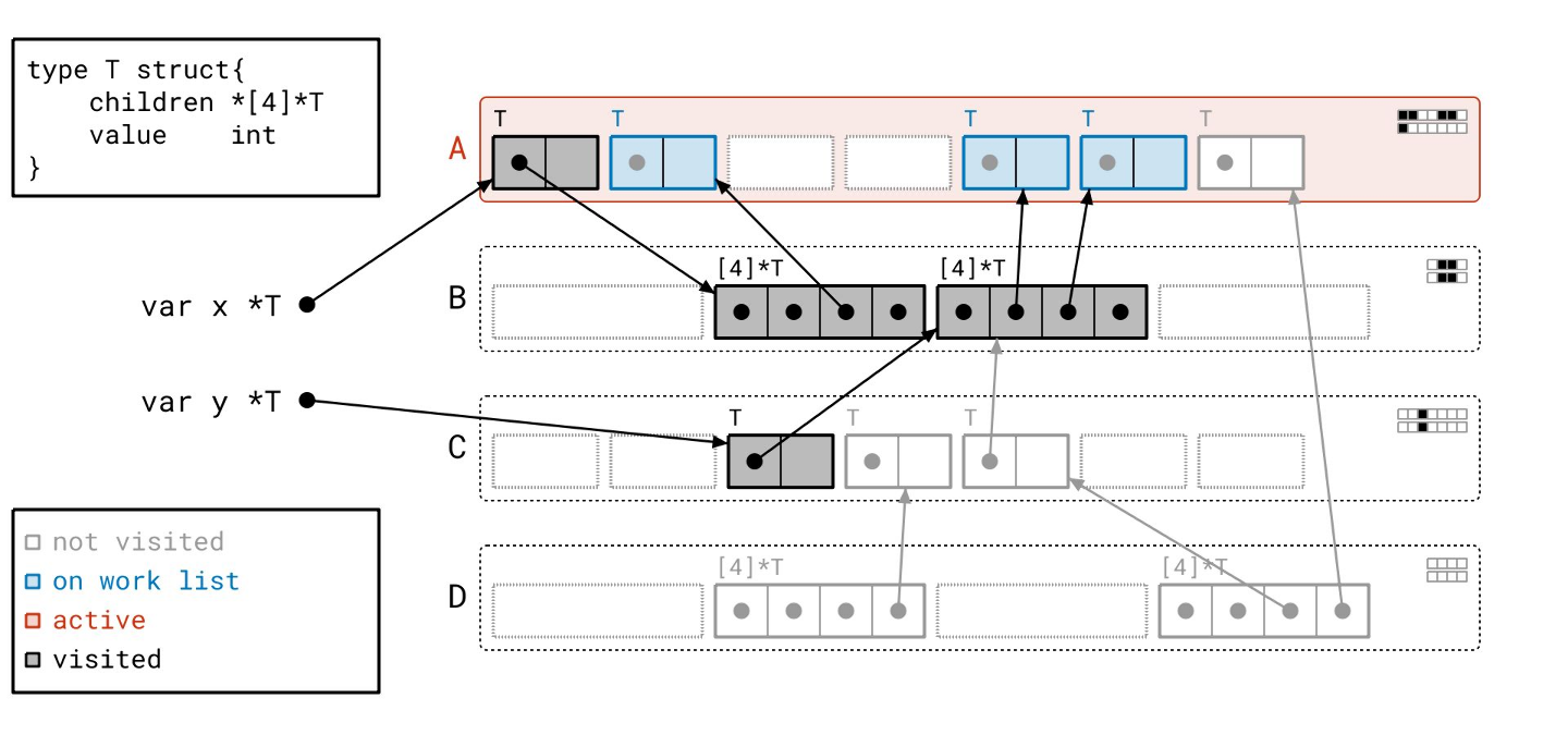
The path the original graph flood took through the heap required 7 separate scans.

We jumped around a whole lot, doing little bits of work in different places. The path taken by Green Tea looks very different.

The path taken by Green Tea requires only 4 scans.

Green Tea, in contrast, makes fewer, longer left-to-right passes over pages A and B. The longer these arrows, the better, and with bigger heaps, this effect can be much stronger. That’s the magic of Green Tea.

It’s also our opportunity to ride the highway.

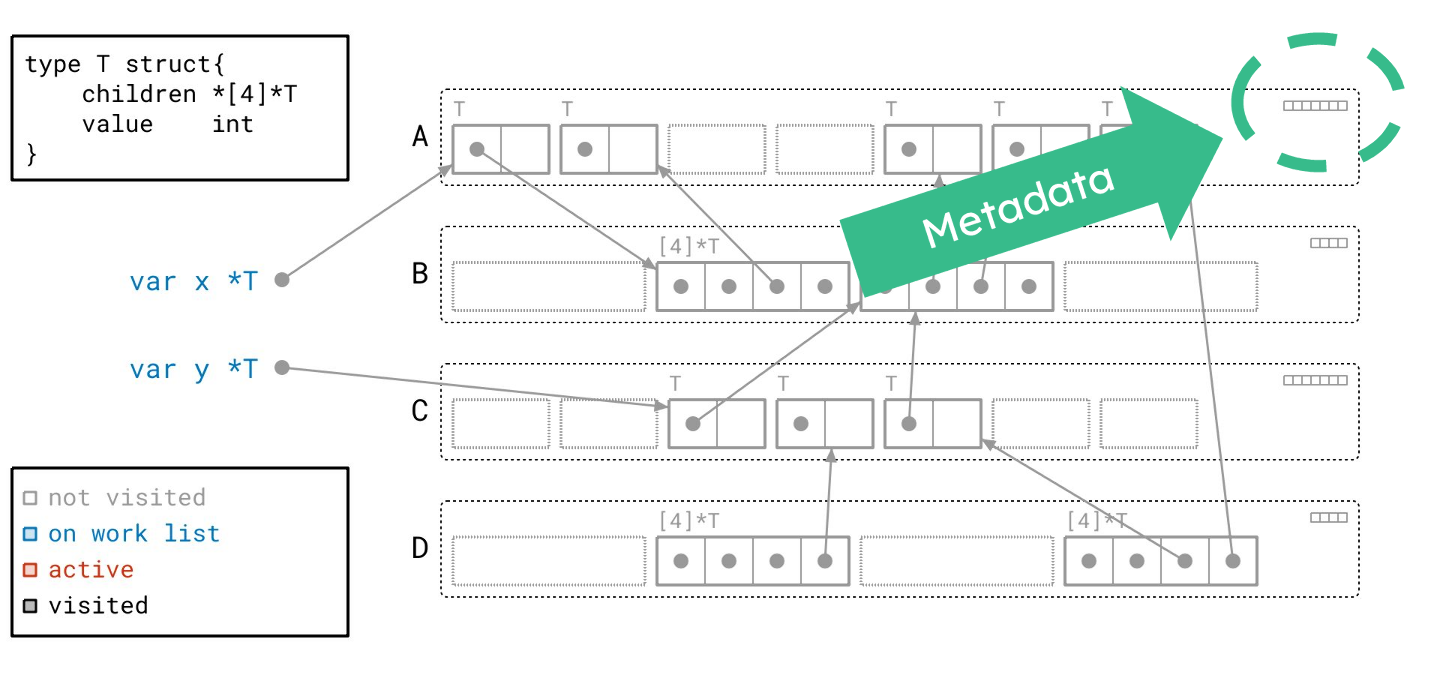
This all adds up to a better fit with the microarchitecture. We can now scan objects closer together with much higher probability, so there’s a better chance we can make use of our caches and avoid main memory. Likewise, per-page metadata is more likely to be in cache. Tracking pages instead of objects means work lists are smaller, and less pressure on work lists means less contention and fewer CPU stalls.

And speaking of the highway, we can take our metaphorical engine into gears we’ve never been able to before, since now we can use vector hardware!

Vector acceleration

If you’re only vaguely familiar with vector hardware, you might be confused as to how we can use it here. But besides the usual arithmetic and trigonometric operations, recent vector hardware supports two things that are valuable for Green Tea: very wide registers, and sophisticated bit-wise operations.

Most modern x86 CPUs support AVX-512, which has 512-bit wide vector registers. This is wide enough to hold all of the metadata for an entire page in just two registers, right on the CPU, enabling Green Tea to work on an entire page in just a few straight-line instructions. Vector hardware has long supported basic bit-wise operations on whole vector registers, but starting with AMD Zen 4 and Intel Ice Lake, it also supports a new bit vector “Swiss army knife” instruction that enables a key step of the Green Tea scanning process to be done in just a few CPU cycles. Together, these allow us to turbo-charge the Green Tea scan loop.

This wasn’t even an option for the graph flood, where we’d be jumping between scanning objects that are all sorts of different sizes. Sometimes you needed two bits of metadata and sometimes you needed ten thousand. There simply wasn’t enough predictability or regularity to use vector hardware.

If you want to nerd out on some of the details, read along! Otherwise, feel free to skip ahead to the evaluation.

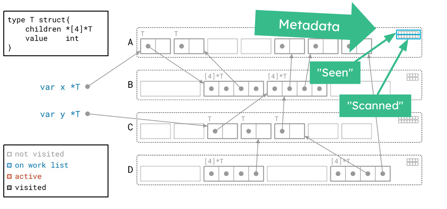
AVX-512 scanning kernel

To get a sense of what AVX-512 GC scanning looks like, take a look at the diagram below.

There’s a lot going on here and we could probably fill an entire blog post just on how this works. For now, let’s just break it down at a high level:

First we fetch the “seen” and “scanned” bits for a page. Recall, these are one bit per object in the page, and all objects in a page have the same size.
Next, we compare the two bit sets. Their union becomes the new “scanned” bits, while their difference is the “active objects” bitmap, which tells us which objects we need to scan in this pass over the page (versus previous passes).
We take the difference of the bitmaps and “expand” it, so that instead of one bit per object, we have one bit per word (8 bytes) of the page. We call this the “active words” bitmap. For example, if the page stores 6-word (48-byte) objects, each bit in the active objects bitmap will be copied to 6 bits in the active words bitmap. Like so:

0 0 1 1 ...

→

000000 000000 111111 111111 ...

Next we fetch the pointer/scalar bitmap for the page. Here, too, each bit corresponds to a word (8 bytes) of the page, and it tells us whether that word stores a pointer. This data is managed by the memory allocator.
Now, we take the intersection of the pointer/scalar bitmap and the active words bitmap. The result is the “active pointer bitmap”: a bitmap that tells us the location of every pointer in the entire page contained in any live object we haven’t scanned yet.
Finally, we can iterate over the memory of the page and collect all the pointers. Logically, we iterate over each set bit in the active pointer bitmap, load the pointer value at that word, and write it back to a buffer that will later be used to mark objects seen and add pages to the work list. Using vector instructions, we’re able to do this 64 bytes at a time, in just a couple instructions.

Part of what makes this fast is the VGF2P8AFFINEQB instruction, part of the “Galios Field New Instructions” x86 extension, and the bit manipulation Swiss army knife we referred to above. It’s the real star of the show, since it lets us do step (3) in the scanning kernel very, very efficiently. It performs a bit-wise affine transformations, treating each byte in a vector as itself a mathematical vector of 8 bits and multiplying it by an 8x8 bit matrix. This is all done over the Galois field GF(2), which just means multiplication is AND and addition is XOR. The upshot of this is that we can define a few 8x8 bit matrices for each object size that perform exactly the 1:n bit expansion we need.

For the full assembly code, see this file. The “expanders” use different matrices and different permutations for each size class, so they’re in a separate file that’s written by a code generator. Aside from the expansion functions, it’s really not a lot of code. Most of it is dramatically simplified by the fact that we can perform most of the above operations on data that sits purely in registers. And, hopefully soon this assembly code will be replaced with Go code!

Credit to Austin Clements for devising this process. It’s incredibly cool, and incredibly fast!

Evaluation

So that’s it for how it works. How much does it actually help?

It can be quite a lot. Even without the vector enhancements, we see reductions in garbage collection CPU costs between 10% and 40% in our benchmark suite. For example, if an application spends 10% of its time in the garbage collector, then that would translate to between a 1% and 4% overall CPU reduction, depending on the specifics of the workload. A 10% reduction in garbage collection CPU time is roughly the modal improvement. (See the GitHub issue for some of these details.)

We’ve rolled Green Tea out inside Google, and we see similar results at scale.

We’re still rolling out the vector enhancements, but benchmarks and early results suggest this will net an additional 10% GC CPU reduction.

While most workloads benefit to some degree, there are some that don’t.

Green Tea is based on the hypothesis that we can accumulate enough objects to scan on a single page in one pass to counteract the costs of the accumulation process. This is clearly the case if the heap has a very regular structure: objects of the same size at a similar depth in the object graph. But there are some workloads that often require us to scan only a single object per page at a time. This is potentially worse than the graph flood because we might be doing more work than before while trying to accumulate objects on pages and failing.

The implementation of Green Tea has a special case for pages that have only a single object to scan. This helps reduce regressions, but doesn’t completely eliminate them.

However, it takes a lot less per-page accumulation to outperform the graph flood than you might expect. One surprise result of this work was that scanning a mere 2% of a page at a time can yield improvements over the graph flood.

Availability

Green Tea is already available as an experiment in the recent Go 1.25 release and can be enabled by setting the environment variable GOEXPERIMENT to greenteagc at build time. This doesn’t include the aforementioned vector acceleration.

We expect to make it the default garbage collector in Go 1.26, but you’ll still be able to opt-out with GOEXPERIMENT=nogreenteagc at build time. Go 1.26 will also add vector acceleration on newer x86 hardware, and include a whole bunch of tweaks and improvements based on feedback we’ve collected so far.

If you can, we encourage you to try at Go tip-of-tree! If you prefer to use Go 1.25, we’d still love your feedback. See this GitHub comment with some details on what diagnostics we’d be interested in seeing, if you can share, and the preferred channels for reporting feedback.

The journey

Before we wrap up this blog post, let’s take a moment to talk about the journey that got us here. The human element of the technology.

The core of Green Tea may seem like a single, simple idea. Like the spark of inspiration that just one single person had.

But that’s not true at all. Green Tea is the result of work and ideas from many people over several years. Several people on the Go team contributed to the ideas, including Michael Pratt, Cherry Mui, David Chase, and Keith Randall. Microarchitectural insights from Yves Vandriessche, who was at Intel at the time, also really helped direct the design exploration. There were a lot of ideas that didn’t work, and there were a lot of details that needed figuring out. Just to make this single, simple idea viable.

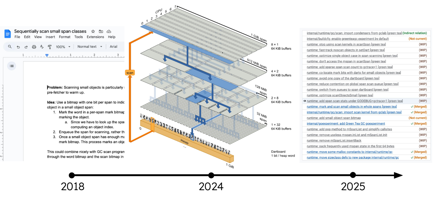
A timeline depicting a subset of the ideas we tried in this vein before getting to where we are today.

The seeds of this idea go all the way back to 2018. What’s funny is that everyone on the team thinks someone else thought of this initial idea.

Green Tea got its name in 2024 when Austin worked out a prototype of an earlier version while cafe crawling in Japan and drinking LOTS of matcha! This prototype showed that the core idea of Green Tea was viable. And from there we were off to the races.

Throughout 2025, as Michael implemented and productionized Green Tea, the ideas evolved and changed even further.

This took so much collaborative exploration because Green Tea is not just an algorithm, but an entire design space. One that we don’t think any of us could’ve navigated alone. It’s not enough to just have the idea, but you need to figure out the details and prove it. And now that we’ve done it, we can finally iterate.

The future of Green Tea is bright.

Once again, please try it out by setting GOEXPERIMENT=greenteagc and let us know how it goes! We’re really excited about this work and want to hear from you!

Previous article: Flight Recorder in Go 1.25
Blog Index